1.4: Lines, Planes, and Hyperplanes

In this section we will add to our basic geometric understanding of \(\mathbb{R}^n\) by studying lines and planes. If we do this carefully, we shall see that working with lines and planes in \(\mathbb{R}^n\) is no more difficult than working with them in \(\mathbb{R}^2\) or \(\mathbb{R}^3\).

Lines in \(\mathbb{R}^n\)

We will start with lines. Recall from Section 1.1 that if \(\mathbf{v}\) is a nonzero vector in \(\mathbb{R}^n\), then, for any scalar \(t\), \(t \mathbf{v}\) has the same direction as \(\mathbf{v}\) when \(t>0\) and the opposite direction when \(t < 0\). Hence the set of points

\[ \{ t\mathbf{v}:-\infty<t<\infty \} \nonumber \]

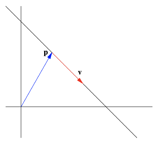
forms a line through the origin. If we now add a vector \(\mathbf{p}\) to each of these points, we obtain the set of points

\[ \{t\mathbf{v}+\mathbf{p}:-\infty<t<\infty \}, \nonumber \]

which is a line through \(\mathbf{p}\) in the direction of \(\mathbf{v}\), as illustrated in Figure 1.4.1 for \(\mathbb{R}^2\).

Figure \(\PageIndex{}\):\PageIndex{1}\): A line in \(\mathbb{R}^2\) through \(\mathbf{p}\) in the direction of \(\mathbf{v}\)

Definition \(\PageIndex{1}\)

Given a vector \(\mathbf{p}\) and a nonzero vector \(\mathbf{v}\) in \(\mathbb{R}^n\), the set of all points \(\mathbf{y}\) in \(\mathbb{R}^n\) such that

\[ \mathbf{y}=t \mathbf{v}+\mathbf{p}, \label{1.4.1} \]

where \(-\infty<t<\infty\), is called the line through \(\mathbf{p}\) in the direction of \(\mathbf{v}\).

Equation (\(\ref{1.4.1}\)) is called a vector equation for the line. If we write \(\mathbf{y}=\left(y_{1}, y_{2}, \ldots, y_{n}\right)\), \(\mathbf{v}=\left(v_{1}, v_{2}, \ldots, v_{n}\right)\), and \(\mathbf{p}=\left(p_{1}, p_{2}, \ldots, p_{n}\right)\), then (1.4.1) may be written as

\[\left(y_{1}, y_{2}, \ldots, y_{n}\right)=t\left(v_{1}, v_{2}, \ldots, v_{n}\right)+\left(p_{1}, p_{2}, \ldots, p_{n}\right) , \label{1.4.2} \]

which holds if and only if

\[\begin{align}
&y_{1}=t v_{1}+p_{1} , \nonumber\\
&y_{2}=t v_{2}+p_{2} , \label{1.4.3} \\
&\vdots \nonumber \\
&y_{n}=t v_{n}+p_{n} . \nonumber
\end{align}\]

The equations in (\(\ref{1.4.3}\)) are called parametric equations for the line.

Example \(\PageIndex{1}\)

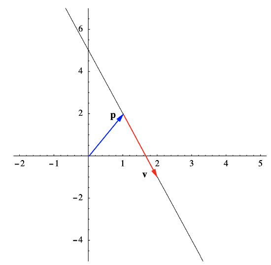
Suppose \(L\) is the line in \(\mathbb{R}^2\) through \(\mathbf{p}=(1,2)\) in the direction of \(\mathbf{v}=(1,-3)\) (see Figure 1.4.2). Then

\[\mathbf{y}=t(1,-3)+(1,2)=(t+1,-3 t+2) \nonumber \]

is a vector equation for \(L\) and, if we let \( \mathbf{y}=(x, y)\),

\[ \begin{aligned}
&x=t+1, \\
&y=-3 t+2
\end{aligned} \]

are parametric equations for \(L\). Note that if we solve for \(t\) in both of these equations, we have

\[ \begin{aligned}
t &=x-1 \\
t &=\frac{2-y}{3} .
\end{aligned}\]

Thus

\[x-1=\frac{2-y}{3} , \nonumber \]

and so

\[y=-3 x+5 . \nonumber \]

Of course, the latter is just the standard slope-intercept form for the equation of a line in \(\mathbb{R}^2\).

Figure \(\PageIndex{}\):\PageIndex{2}\): The line through \(\mathbf{p} = (1,2) \) in the direction of \(\mathbf{v} =(1,-3)\)

Example \(\PageIndex{2}\)

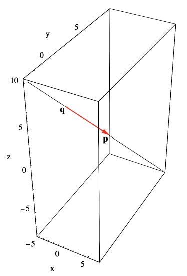
Now suppose we wish to find an equation for the line L in \(\mathbb{R}^3\) which passes through the points \(\mathbf{p}=(1,3,1)\) and \(\mathbf{q}=(-1,1,4)\) (see Figure 1.4.3). We first note that the vector

\[\mathbf{p}-\mathbf{q}=(2,2,-3) \nonumber \]

gives the direction of the line, so

\[\mathbf{y}=t(2,2,-3)+(1,3,1) \nonumber \]

is a vector equation for \(L\); if we let \(\mathbf{y}=(x, y, z)\),

\[\begin{aligned}
&x=2 t+1 , \\
&y=2 t+3 , \\
&z=-3 t+1
\end{aligned}\]

are parametric equations for \(L\).

Figure \(\PageIndex{}\):\PageIndex{3}\): The line through \(\mathbf{p}=(1,3,1)\) and \(\mathbf{q}=(-1,1,4)\)

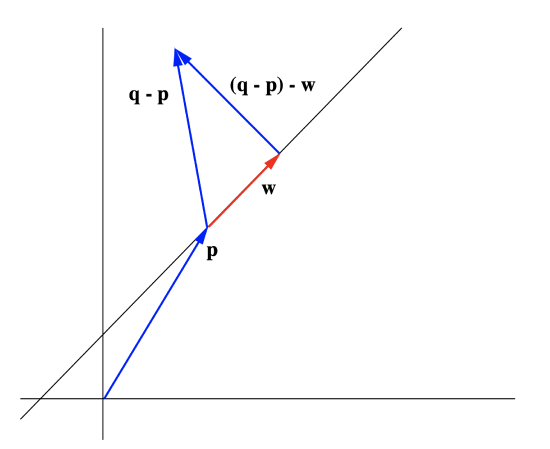
As an application of these ideas, consider the problem of finding the shortest distance from a point \( \mathbf{q}\) in \(\mathbb{R}^n\) to a line L with equation \(\mathbf{y}=t \mathbf{v}+\mathbf{p}\). If we let \( \mathbf{w}\) be the projection of \(\mathbf{q}-\mathbf{p}\) onto \( \mathbf{v}\), then, as we saw in Section 1.2, the vector \((\mathbf{q}-\mathbf{p})-\mathbf{w}\) is orthogonal to \(\mathbf{v}\) and may be pictured with its tail on \(L\) and its tip at \(\mathbf{q}\). Hence the shortest distance from \(\mathbf{q}\) to \(L\) is \(\|(\mathbf{q}- \mathbf{p}) − \mathbf{w}\|\). See Figure 1.4.4.

Figure \(\PageIndex{}\):\PageIndex{4}\): Distance from a point \( \mathbf{q}\) to a line

Example \(\PageIndex{3}\)

To find the distance from the point \(\mathbf{q}=(2,2,4)\) to the line \(L\) through the points \(\mathbf{p}=(1,0,0)\) and \(\mathbf{r}=(0,1,0)\), we must first find an equation for \(L\). Since the direction of \(L\) is given by \(\mathbf{v}=\mathbf{r}-\mathbf{p}=(-1,1,0)\), a vector equation for \(L\) is

\[\mathbf{y}=t(-1,1,0)+(1,0,0) . \nonumber \]

If we let

\[ \mathbf{u}=\frac{\mathbf{v}}{\|\mathbf{v}\|}=\frac{1}{\sqrt{2}}(-1,1,0) , \nonumber \]

then the projection of \(\mathbf{q}-\mathbf{p}\) onto \(\mathbf{v}\) is

\[\begin{equation}
\left.\mathbf{w}=((\mathbf{q}-\mathbf{p}) \cdot \mathbf{u}) \mathbf{u}=\left((1,2,4) \cdot \frac{1}{\sqrt{2}}(-1,1,0)\right)\right) \frac{1}{\sqrt{2}}(-1,1,0)=\frac{1}{2}(-1,1,0) .
\end{equation} \nonumber \]

Thus the distance from \(\mathbf{q}\) to \(L\) is

\[\begin{equation}
\|(\mathbf{q}-\mathbf{p})-\mathbf{w}\|=\left\|\left(\frac{3}{2}, \frac{3}{2}, 4\right)\right\|=\sqrt{\frac{82}{4}}=\sqrt{20.5} .
\end{equation} \nonumber \]

Definition \(\PageIndex{2}\)

Suppose \(L\) and \(M\) are lines in \(\mathbb{R}^n\) with equations \(\begin{equation}
\mathbf{y}=t \mathbf{v}+\mathbf{p}
\end{equation}\) and \(\begin{equation}
\mathbf{y}=t \mathbf{w}+\mathbf{q}
\end{equation}\), respectively. We say \(L\) and \(M\) are parallel if \(\mathbf{v}\) and \(\mathbf{w}\) are parallel. We say \(L\) and \(M\) are perpendicular, or orthogonal, if they intersect and \(\mathbf{v}\) and \(\mathbf{w}\) are orthogonal.

Note that, by definition, a line is parallel to itself.

Figure \(\PageIndex{}\):\PageIndex{5}\): Parallel (\(L\) and \(M\)) and perpendicular (\(L\) and \(N\)) lines

Example \(\PageIndex{4}\)

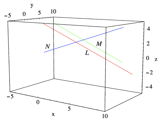
The lines \(L\) and \(M\) in \(\mathbb{R}^3\) with equations

\[\begin{equation}
\mathbf{y}=t(1,2,-1)+(4,1,2)
\end{equation} \nonumber \]

and

\[\mathbf{y}=t(-2,-4,2)+(5,6,1) , \nonumber \]

respectively, are parallel since (−2,−4,2) = −2(1,2,−1), that is, the vectors (1,2,−1) and (−2,−4,2) are parallel. See Figure 1.4.5.

Example \(\PageIndex{5}\)

The lines \(L\) and \(N\) in \(\mathbb{R}^3\) with equations

\[\mathbf{y}=t(1,2,-1)+(4,1,2) \nonumber \]

and

\[\mathbf{y}=t(3,-1,1)+(-1,5,-1) , \nonumber \]

respectively, are perpendicular since they intersect at (5,3,1) (when \(t=1\) for the first line and \(t=2\) for the second line) and (1,2,−1) and (3,−1,1) are orthogonal since

\[(1,2,-1) \cdot(3,-1,1)=3-2-1=0 . \nonumber \]

See Figure 1.4.5.

Planes in \(\mathbb{R}^n\)

The following definition is the first step in defining a plane.

Definition \(\PageIndex{3}\)

Two vectors \(\mathbf{x}\) and \(\mathbf{y}\) in \(\mathbb{R}^n\) are said to be linearly independent if neither one is a scalar multiple of the other.

Geometrically, \(\mathbf{x}\) and \(\mathbf{y}\) are linearly independent if they do not lie on the same line through the origin. Notice that for any vector \(\mathbf{x}\), \(\mathbf{0}\) and \(\mathbf{x}\) are not linearly independent, that is, they are linearly dependent, since \(\mathbf{0}=0 \mathbf{x}\).

Definition \(\PageIndex{4}\)

Given a vector \(\mathbf{p}\) along with linearly independent vectors \(\mathbf{v}\) and \(\mathbf{w}\), all in \(\mathbb{R}^n\), the set of all points \(\mathbf{y}\) such that

\[\mathbf{y}=t \mathbf{v}+s \mathbf{w}+\mathbf{p}, \label{1.4.4}\]

where \(-\infty<t<\infty\) and \(-\infty<s<\infty\), is called a plane.

The intuition here is that a plane should be a two dimensional object, which is guaranteed because of the requirement that \(\mathbf{v}\) and \(\mathbf{w}\) are linearly independent. Also note that if we let \(\mathbf{y}=\left(y_{1}, y_{2}, \ldots, y_{n}\right)\), \(\mathbf{v}=\left(v_{1}, v_{2}, \ldots, v_{n}\right)\), \(\mathbf{w}=\left(w_{1}, w_{2}, \ldots, w_{n}\right)\), and \(\mathbf{p}=\left(p_{1}, p_{2}, \ldots, p_{n}\right)\), then (\(\ref{1.4.4}\)) implies that

\[\begin{align}
y_{1}=t v_{1}+s w_{1}+p_{1} , \nonumber \\
y_{2}=t v_{2}+s w_{2}+p_{2} , \nonumber \\
\vdots \quad \vdots \label{1.4.5} \\
y_{n}=t v_{n}+s w_{n}+p_{n} . \nonumber
\end{align}\]

As with lines, (\(\ref{1.4.4}\)) is a vector equation for the plane and the equations in (\(\ref{1.4.5}\)) are parametric equations for the plane.

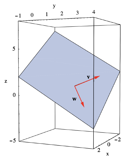
Example \(\PageIndex{6}\)

Suppose we wish to find an equation for the plane P in \(\mathbb{R}^3\) which contains the three points \(\mathbf{p}=(1,2,1)\), \(\mathbf{q}=(-1,3,2)\), and \(\mathbf{r}=(2,3,-1)\). The first step is to find two linearly independent vectors \(\mathbf{v}\) and \(\mathbf{w}\) which lie in the plane. Since \(P\) must contain the line segments from \(\mathbf{p}\) to \(\mathbf{q}\) and from \(\mathbf{p}\) to \(\mathbf{r}\), we can take \[\mathbf{v}=\mathbf{q}-\mathbf{p}=(-2,1,1)\nonumber \]

and

\[\mathbf{w}=\mathbf{r}-\mathbf{p}=(1,1,-2) . \nonumber \]

Note that \(\mathbf{v}\) and \(\mathbf{w}\) are linearly independent, a consequence of \(\mathbf{p}\), \(\mathbf{q}\), and \(\mathbf{r}\) not all lying on the same line. See Figure 1.4.6. We may now write a vector equation for \(P\) as

\[\mathbf{y}=t(-2,1,1)+s(1,1,-2)+(1,2,1) . \nonumber \]

Note that \(\mathbf{y}=\mathbf{p}\) when \(t=0\) and \(s=0\), \(\mathbf{y}=\mathbf{q}\) when \(t=1\) and \(s=0\), and \(\mathbf{y}=\mathbf{r}\) when \(t=0\) and \(s=1\). If we write \(\mathbf{y}=(x, y, z)\), then, expanding the vector equation,

\[(x, y, z)=t(-2,1,1)+s(1,1,-2)+(1,2,1)=(-2 t+s+1, t+s+2, t-2 s+1) , \nonumber \]

giving us \[\begin{aligned}
&x=-2 t+s+1, \\
&y=t+s+2 , \\
&z=t-2 s+1
\end{aligned}\]

for parametric equations for \(P\).

Figure \(\PageIndex{}\):\PageIndex{6}\): The plane \(\mathbf{y}=t \mathbf{v}+s \mathbf{w}+\mathbf{p}\), with \(\mathbf{v}=(-2,1,1), \mathbf{w}=(1,1,-2), \mathbf{p}=(1,2,1)\)

To find the shortest distance from a point \(\mathbf{q}\) to a plane \(P\), we first need to consider the problem of finding the projection of a vector onto a plane. To begin, consider the plane \(P\) through the origin with equation \(\mathbf{y}=t \mathbf{a}+s \mathbf{b}\) where \(\|a\|=1\), \(\|b\|=1\), and \(\mathbf{a} \perp \mathbf{b}\). Given a vector \(\mathbf{q}\) not in \(P\), let

\[\mathbf{r}=(\mathbf{q} \cdot \mathbf{a}) \mathbf{a}+(\mathbf{q} \cdot \mathbf{b}) \mathbf{b} , \nonumber \]

the sum of the projections of \(\mathbf{q}\) onto \(\mathbf{a}\) and onto \(\mathbf{b}\). Then

\[\begin{aligned}
(\mathbf{q}-\mathbf{r}) \cdot \mathbf{a} &=\mathbf{q} \cdot \mathbf{a}-\mathbf{r} \cdot \mathbf{a} \\
&=\mathbf{q} \cdot \mathbf{a}-(\mathbf{q} \cdot \mathbf{a})(\mathbf{a} \cdot \mathbf{a})-(\mathbf{q} \cdot \mathbf{b})(\mathbf{b} \cdot \mathbf{a}) \\
&=\mathbf{q} \cdot \mathbf{a}-\mathbf{q} \cdot \mathbf{a}=0,
\end{aligned}\]

since \(\mathbf{a} \cdot \mathbf{a}=\|a\|^{2}=1\) and \(\mathbf{b} \cdot \mathbf{a}=0\), and, similarly,

\[\begin{aligned}
(\mathbf{q}-\mathbf{r}) \cdot \mathbf{b} &=\mathbf{q} \cdot \mathbf{b}-\mathbf{r} \cdot \mathbf{b} \\
&=\mathbf{q} \cdot \mathbf{b}-(\mathbf{q} \cdot \mathbf{a})(\mathbf{a} \cdot \mathbf{b})-(\mathbf{q} \cdot \mathbf{b})(\mathbf{b} \cdot \mathbf{b}) \\
&=\mathbf{q} \cdot \mathbf{b}-\mathbf{q} \cdot \mathbf{b}=0.
\end{aligned}\]

It follows that for any \(\mathbf{y}=t \mathbf{a}+s \mathbf{b}\) in the plane P,

\[(\mathbf{q}-\mathbf{r}) \cdot \mathbf{y}=(\mathbf{q}-\mathbf{r}) \cdot(t \mathbf{a}+s \mathbf{b})=t(\mathbf{q}-\mathbf{r}) \cdot \mathbf{a}+s(\mathbf{q}-\mathbf{r}) \cdot \mathbf{b}=0 . \nonumber \]

That is, \(\mathbf{q}-\mathbf{r}\) is orthogonal to every vector in the plane \(P\). For this reason, we call \(\mathbf{r}\) the projection of \(\mathbf{q}\) onto the plane \(P\), and we note that the shortest distance from \(\mathbf{q}\) to \(P\) is \(\|\mathbf{q}-\mathbf{r}\|\).

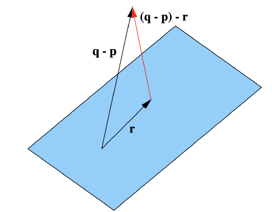
In the general case, given a point \(\mathbf{q}\) and a plane \(P\) with equation \(\mathbf{y}=t \mathbf{v}+s \mathbf{w}+\mathbf{p}\), we need only find vectors \(\mathbf{a}\) and \(\mathbf{b}\) such that \(\mathbf{a} \perp \mathbf{b}\), \(\|a\|=1\), \(\|b\|=1\), and the equation \(\mathbf{y}=t \mathbf{a}+s \mathbf{b}+\mathbf{p}\) describes the same plane \(P\). You are asked in Exercise 29 to verify that if we let \(\mathbf{c}\) be the projection of \(\mathbf{w}\) onto \(\mathbf{v}\), then we may take

\[\mathbf{a}=\frac{1}{\|\mathbf{v}\|} \mathbf{v} \nonumber \]

and

\[\mathbf{b}=\frac{1}{\|\mathbf{w}-\mathbf{c}\|}(\mathbf{w}-\mathbf{c}) . \nonumber \]

If \(\mathbf{r}\) is the sum of the projections of \(\mathbf{q}-\mathbf{p}\) onto \(\mathbf{a}\) and \(\mathbf{b}\), then r is the projection of \(\mathbf{q}-\mathbf{p}\) onto \(P\) and \(\|(\mathbf{q}-\mathbf{p})-\mathbf{r}\| \) is the shortest distance from \(\mathbf{q}\) to \(P\). See Figure 1.4.7.

Figure \(\PageIndex{}\):\PageIndex{7}\): Distance from a point \(\mathbf{q}\) to a plane

Example \(\PageIndex{7}\)

To compute the distance from the point \(\mathbf{q}=(2,3,3)\) to the plane \(P\) with equation

\[\mathbf{y}=t(-2,1,0)+s(1,-1,1)+(-1,2,1) , \nonumber \]

let \(\mathbf{v}=(-2,1,0)\), \(\mathbf{w}=(1,-1,1)\), and \(\mathbf{p}=(-1,2,1)\). Then, using the above notation, we have

\[\begin{gathered}
\mathbf{a}=\frac{1}{\sqrt{5}}(-2,1,0) , \\
\mathbf{c}=(\mathbf{w} \cdot \mathbf{a}) \mathbf{a}=-\frac{3}{5}(-2,1,0) ,
\end{gathered} \]

\[ \mathbf{w}-\mathbf{c}=\frac{1}{5}(-1,-2,5) , \nonumber \]

and

\[\mathbf{b}=\frac{1}{\sqrt{30}}(-1,-2,5) . \nonumber \]

Since \(\mathbf{q}-\mathbf{p}=(3,1,2)\), the projection of \(\mathbf{q}-\mathbf{p}\) onto \(P\) is

\[\mathbf{r}=((3,1,2) \cdot \mathbf{a}) \mathbf{a}+((3,1,2) \cdot \mathbf{b}) \mathbf{b}=-(-2,1,0)+\frac{1}{6}(-1,-2,5)=\frac{1}{6}(11,-8,5) \nonumber \]

and

\[(\mathbf{q}-\mathbf{p})-\mathbf{r}=\frac{1}{6}(7,14,7) . \nonumber \]

Hence the distance from \(\mathbf{q}\) to \(P\) is

\[\|(\mathbf{q}-\mathbf{p})-\mathbf{r}\|=\frac{\sqrt{294}}{6}=\frac{7}{\sqrt{6}} . \nonumber \]

More generally, we say vectors \(\mathbf{v}_{1}, \mathbf{v}_{2}, \ldots, \mathbf{v}_{k}\) in \(\mathbb{R}^n\) are linearly independent if no one of them can be written as a sum of scalar multiples of the others. Given a vector \(\mathbf{p}\) and linearly independent vectors \(\mathbf{v}_{1}, \mathbf{v}_{2}, \ldots, \mathbf{v}_{k}\) we call the set of all points \(\mathbf{y}\) such that

\[ \mathbf{y}=t_{1} \mathbf{v}_{1}+t_{2} \mathbf{v}_{2}+\cdots+t_{k} \mathbf{v}_{k}+\mathbf{p}, \nonumber \]

where \(-\infty<t_{j}<\infty\), \(j=1,2, \ldots, k\), a k-dimensional affine subspace of \(\mathbb{R}^n\). In this terminology, a line is a 1-dimensional affine subspace and a plane is a 2-dimensional affine subspace. In the following, we will be interested primarily in lines and planes and so will not develop the details of the more general situation at this time.

Hyperplanes

Consider the set \(L\) of all points \(\mathbf{y}=(x, y)\) in \(\mathbb{R}^2\) which satisfy the equation

\[ a x+b y+d=0 , \label{1.4.6} \]

where \(a\), \(b\), and \(d\) are scalars with at least one of \(a\) and \(b\) not being 0. If, for example, \(b \neq 0\), then we can solve for \(y\), obtaining

\[y=-\frac{a}{b} x-\frac{d}{b} . \label{1.4.7} \]

If we set \(x = t\), \(-\infty<t<\infty\), then the solutions to (\(\ref{1.4.6}\)) are

\[\mathbf{y}=(x, y)=\left(t,-\frac{a}{b} t-\frac{d}{b}\right)=t\left(1,-\frac{a}{b}\right)+\left(0,-\frac{d}{b}\right). \label{1.4.8}\]

Thus \(L\) is a line through \(\left(0,-\frac{d}{b}\right)\) in the direction of \(\left(1,-\frac{a}{b}\right)\). A similar calculation shows that if \(a \neq 0\), then we can describe \(L\) as the line through \( \left(-\frac{d}{a}, 0\right) \) in the direction of \( \left(-\frac{b}{a}, 1\right) \). Hence in either case \(L\) is a line in \( \mathbb{R}^2 \).

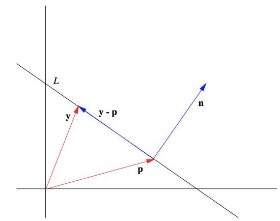
Now let \(\mathbf{n}=(a, b)\) and note that (\(\ref{1.4.6}\)) is equivalent to

\[ \mathbf{n} \cdot \mathbf{y}+d=0 . \label{1.4.9} \]

Moreover, if \(\mathbf{p}=\left(p_{1}, p_{2}\right)\) is a point on \(L\), then

\[ \mathbf{n} \cdot \mathbf{p}+d=0, \label{1.4.10} \]

which implies that \(d=-\mathbf{n} \cdot \mathbf{p} \). Thus we may write (\(\ref{1.4.9}\)) as

\[ \mathbf{n} \cdot \mathbf{y}-\mathbf{n} \cdot \mathbf{p}=0 \nonumber \]

and so we see that (\(\ref{1.4.6}\)) is equivalent to the equation

\[ \mathbf{n} \cdot(\mathbf{y}-\mathbf{p})=0 . \label{1.4.11} \]

Equation (\(\ref{1.4.11}\)) is a normal equation for the line \(L\) and \(\mathbf{n}\) is a normal vector for \(L\). In words, (\(\ref{1.4.11}\)) says that the line \(L\) consists of all points in \( \mathbb{R}^2 \) whose difference with \(\mathbf{p}\) is orthogonal to \(\mathbf{n}\). See Figure 1.4.8.

Figure \(\PageIndex{}\):\PageIndex{8}\): \(L\) is the set of points \(\mathbf{y}\) for which \(\mathbf{y}-\mathbf{p}\) is orthogonal to \(\mathbf{n}\)

Example \(\PageIndex{8}\)

Suppose \(L\) is a line in \(\mathbb{R}^2\) with equation

\[ 2 x+3 y=1 . \nonumber \]

Then a normal vector for \(L\) is \(\mathbf{n}=(2,3)\); to find a point on \(L\), we note that when \(x=2\), \(y=-1\), so \(\mathbf{p}=(2,-1)\) is a point on \(L\). Thus

\[ (2,3) \cdot((x, y)-(2,-1))=0, \nonumber \]

or, equivalently,

\[(2,3) \cdot(x-2, y+1)=0, \nonumber \]

is a normal equation for \(L\). Since \(\mathbf{q}=(-1,1)\) is also a point on \(L\), \(L\) has direction \(\mathbf{q}-\mathbf{p}=(-3,2)\). Thus

\[ \mathbf{y}=t(-3,2)+(2,-1) \nonumber \]

is a vector equation for \(L\). Note that

\[ \mathbf{n} \cdot(\mathbf{q}-\mathbf{p})=(2,3) \cdot(-3,2)=0, \nonumber \]

so \(\mathbf{n}\) is orthogonal to \(\mathbf{q}-\mathbf{p}\).

Example \(\PageIndex{9}\)

If \(L\) is a line in \(\mathbb{R}^2\) through \(\mathbf{p}=(2,3)\) in the direction of \(\mathbf{v}=(-1,2)\), then \(\mathbf{n}=(2,1)\) is a normal vector for \(L\) since \(\mathbf{v} \cdot \mathbf{n}=0 \). Thus

\[ (2,1) \cdot(x-2, y-3)=0 \nonumber \]

is a normal equation for \(L\). Multiplying this out, we have

\[ 2(x-2)+(y-3)=0 ; \nonumber \]

that is, \(L\) consists of all points \((x,y)\) in \(\mathbb{R}^2\) which satisfy

\[ 2 x+y=7 \text { . } \nonumber \]

Now consider the case where \(P\) is the set of all points \(\mathbf{y}=(x, y, z)\) in \(\mathbb{R}^3\) that satisfy the equation

\[ a x+b y+c z+d=0 , \label{1.4.12} \]

where \(a\), \(b\), \(c\), and \(d\) are scalars with at least one of \(a\), \(b\), and \(c\) not being 0. If for example, \(a \neq 0\), then we may solve for \(x\) to obtain

\[ x=-\frac{b}{a} y-\frac{c}{a} z-\frac{d}{a}. \label{1.4.13} \]

If we set \( y=t \),\(-\infty<t<\infty \), and \(z = s\), \(-\infty<s<\infty \), the solutions to (\(\ref{1.4.12}\)) are

\[ \begin{align}
\mathbf{y} &=(x, y, z) \nonumber \\
&=\left(-\frac{b}{a} t-\frac{c}{a} s-\frac{d}{a}, t, s\right) \label{1.4.14} \\
&=t\left(-\frac{b}{a}, 1,0\right)+s\left(-\frac{c}{a}, 0,1\right)+\left(-\frac{d}{a}, 0,0\right) . \nonumber
\end{align} \]

Thus we see that \(P\) is a plane in \(\mathbb{R}^3\). In analogy with the case of lines in \(\mathbb{R}^2\), if we let \(\mathbf{n}=(a, b, c)\) and let \(\mathbf{p}=\left(p_{1}, p_{2}, p_{3}\right)\) be a point on \(P\), then we have

\[ \mathbf{n} \cdot \mathbf{p} + d = ax+bby+cz+d=0 , \nonumber \]

from which we see that \( \mathbf{n} \cdot \mathbf{p} = -d\), and so we may write (\(\ref{1.4.12}\)) as

\[ \mathbf{n} \cdot (\mathbf{y} - \mathbf{p} ) =0 . \label{1.4.15} \]

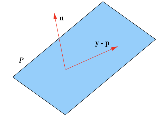
We call (\(\ref{1.4.15}\)) a normal equation for \(P\) and we call \(\mathbf{n}\) a normal vector for \(P\). In words, (\(\ref{1.4.15}\)) says that the plane \(P\) consists of all points in \(\mathbb{R}^3\) whose difference with \(\mathbf{p}\) is orthogonal to \(\mathbf{n}\). See Figure 1.4.9.

Figure \(\PageIndex{}\):\PageIndex{9}\): \(P\) is the set of points \(\mathbf{y}\) for which \(\mathbf{y}-\mathbf{p}\) is orthogonal to \(\mathbf{n}\)

Example \(\PageIndex{10}\)

Let \(P\) be the plane in \(\mathbb{R}^3\) with vector equation

\[ \mathbf{y} = t(2,2,-1) + s(-1,2,1) + (1,1,2) . \nonumber\]

If we let \(\mathbf{v}=(2,2,-1)\) and \(\mathbf{w}=(-1,2,1)\), then

\[ \mathbf{n} = \mathbf{v} \times \mathbf{w} = (4,-1,6) \nonumber \]

is orthogonal to both \(\mathbf{v}\) and \(\mathbf{w}\). Now if \(\mathbf{y}\) is on \(P\), then

\[ \mathbf{y} = t \mathbf{v} + s \mathbf{w} + \mathbf{p} \nonumber \]

for some scalars \(t\) and \(s\), from which we see that

\[ \mathbf{n} \cdot ( \mathbf{y} - \mathbf{p} ) = \mathbf{n} \cdot (t \mathbf{v} + s \mathbf{w}) = t( \mathbf{n} \cdot \mathbf{v} ) + s ( \mathbf{n} \cdot \mathbf{w} ) = 0+0 = 0 . \nonumber \]

That is, \(\mathbf{n}\) is a normal vector for \(P\). So, letting \(\mathbf{y}=(x, y, z)\),

\[ (4,-1,6) \cdot (x - 1, y-1,z-2) = 0 \label{1.4.16} \]

is a normal equation for \(P\). Multiplying (\(\ref{1.4.16}\)) out, we see that \(P\) consists of all points \((x,y,z)\) in \(\mathbb{R}^3\) which satisfy

\[ 4x-y+6z=15 . \nonumber \]

Example \(\PageIndex{11}\)

Suppose \(\mathbf{p}=(1,2,1)\), \(\mathbf{q}=(-2,-1,3)\), and \(\mathbf{r}=(2,-3,-1)\) are three points on a plane \(P\) in \(\mathbb{R}^3\). Then

\[ \mathbf{v} = \mathbf{q} - \mathbf{p} = (-3,-3,2) \nonumber \]

and

\[\mathbf{w} = \mathbf{r} - \mathbf{p} = (1,-5,-2) \nonumber \]

are vectors lying on \(P\). Thus

\[ \mathbf{n}=\mathbf{v} \times \mathbf{w}=(16,-4,18) \nonumber \]

is a normal vector for \(P\). Hence

\[ (16,-4,18) \cdot (x-1,y-2,z-1)=0 \nonumber \]

is a normal equation for \(P\). Thus \(P\) is the set of all points \((x,y,z)\) in \(\mathbb{R}^3\) satisfying

\[ 16 x-4 y+18 y=26 . \nonumber \]

The following definition generalizes the ideas in the previous examples.

Definition \(\PageIndex{5}\)

Suppose \(\mathbf{n}\) and \(\mathbf{p}\) are vectors in \(\mathbb{R}^n\) with \(\mathbf{n} \neq \mathbf{0} \). The set of all vectors \(\mathbf{y}\) in \(\mathbb{R}^n\) which satisfy the equation

\[ \mathbf{n} \cdot(\mathbf{y}-\mathbf{p})=0 \label{1.4.17} \]

is called a hyperplane through the point \(\mathbf{p}\). We call \(\mathbf{n}\) a normal vector for the hyperplane and we call (\(\ref{1.4.17}\)) a normal equation for the hyperplane.

In this terminology, a line in \(\mathbb{R}^2\) is a hyperplane and a plane in \(\mathbb{R}^3\)is a hyperplane. In general, a hyperplane in \(\mathbb{R}^n\) is an (n − 1)-dimensional affine subspace of \(\mathbb{R}^n\) . Also, note that if we let \(\mathbf{n}=\left(a_{1}, a_{2}, \ldots, a_{n}\right)\), \(\mathbf{p}=\left(p_{1}, p_{2}, \ldots, p_{n}\right)\), and \(\mathbf{y}=\left(y_{1}, y_{2}, \ldots, y_{n}\right)\), then we may write (\(\ref{1.4.17}\)) as

\[a_{1}\left(y_{1}-p_{1}\right)+a_{2}\left(y_{2}-p_{2}\right)+\cdots+a_{n}\left(y_{n}-p_{n}\right)=0 , \label{1.4.18} \]

or

\[ a_{1} y_{1}+a_{2} y_{2}+\cdots+a_{n} y_{n}+d=0 \label{1.4.19} \]

where \( d=-\mathbf{n} \cdot \mathbf{p} . \)

Example \(\PageIndex{12}\)

The set of all points \((w,x,y,z)\) in \(\mathbb{R}^4\) which satisfy

\[ 3 w-x+4 y+2 z=5 \nonumber \]

is a 3-dimensional hyperplane with normal vector \(\mathbf{n}=(3,-1,4,2)\).

Figure \(\PageIndex{}\):\PageIndex{10}\): Distance from a point \(\mathbf{q}\) to a hyperplane \(H\)

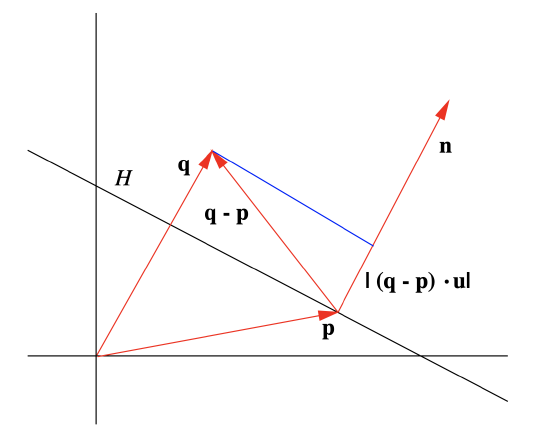
The normal equation description of a hyperplane simplifies a number of geometric calculations. For example, given a hyperplane \(H\) through \(\mathbf{p}\) with normal vector \(\mathbf{n}\) and a point \(\mathbf{q}\) in \(\mathbb{R}^n\), the distance from \(\mathbf{q}\) to \(H\) is simply the length of the projection of \(\mathbf{q}-\mathbf{p}\) onto \(\mathbf{n}\). Thus if \(\mathbf{u}\) is the direction of \(\mathbf{n}\), then the distance from \(\mathbf{q}\) to \(H\) is \(|(\mathbf{q}-\mathbf{p}) \cdot \mathbf{u}| \). See Figure 1.4.10. Moreover, if we let \( d=-\mathbf{p} \cdot \mathbf{n} \)as in (\(\ref{1.4.19}\)), then we have

\[ |(\mathbf{q}-\mathbf{p}) \cdot \mathbf{u}|=|\mathbf{q} \cdot \mathbf{u}-\mathbf{p} \cdot \mathbf{u}|=\frac{\mathbf{q} \cdot \mathbf{n}-\mathbf{p} \cdot \mathbf{n}}{\|\mathbf{n}\|}=\frac{|\mathbf{q} \cdot \mathbf{n}+d|}{\|\mathbf{n}\|} . \label{1.4.20} \]

Note that, in particular, (\(\ref{1.4.20}\)) may be used to find the distance from a point to a line in \(\mathbb{R}^2\) and from a point to a plane in \(\mathbb{R}^3\).

Example \(\PageIndex{13}\)

To find the distance from the point \(\mathbf{q}=(2,3,3)\) to the plane \(P\) in \(\mathbb{R}^3\) with equation

\[ x+2 y+z=4 , \nonumber \]

we first note that \(\mathbf{n}=(1,2,1)\) is a normal vector for \(P\). Using (\(\ref{1.4.20}\)) with \(d = −4\), we see that the distance from \(\mathbf{q}\) to \(P\) is

\[ \frac{|\mathbf{q} \cdot \mathbf{n}+d|}{\|\mathbf{n}\|}=\frac{|(2,3,3) \cdot(1,2,1)-4|}{\sqrt{6}}=\frac{7}{\sqrt{6}} . \nonumber \]

Note that this agrees with an earlier example.

We will close this section with a few words about angles between hyperplanes. Note that a hyperplane does not have a unique normal vector. In particular, if \(\mathbf{n}\) is a normal vector for a hyperplane \(H\), then \(-\mathbf{n}\) is also a normal vector for \(H\). Hence it is always possible to choose the normal vectors required in the following definition.

Definition \(\PageIndex{6}\)

Let \(G\) and \(H\) be hyperplanes in \(\mathbb{R}^n\) with normal equations

\[ \mathbf{m} \cdot(\mathbf{y}-\mathbf{p})=0 \nonumber \]

and

\[ \mathbf{n} \cdot(\mathbf{y}-\mathbf{q})=0 , \nonumber \]

respectively, chosen so that \(\mathbf{m} \cdot \mathbf{n} \geq 0 \). Then the angle between \(G\) and \(H\) is the angle between \(\mathbf{m}\) and \(\mathbf{n}\). Moreover, we will say that \(G\) and \(H\) are orthogonal if \(\mathbf{m}\) and \(\mathbf{n}\) are orthogonal and we will say \(G\) and \(H\) are parallel if \(\mathbf{m}\) and \(\mathbf{n}\) are parallel.

The effect of the choice of normal vectors in the definition is to make the angle between the two hyperplanes be between 0 and \( \frac{ \pi}{2} \)

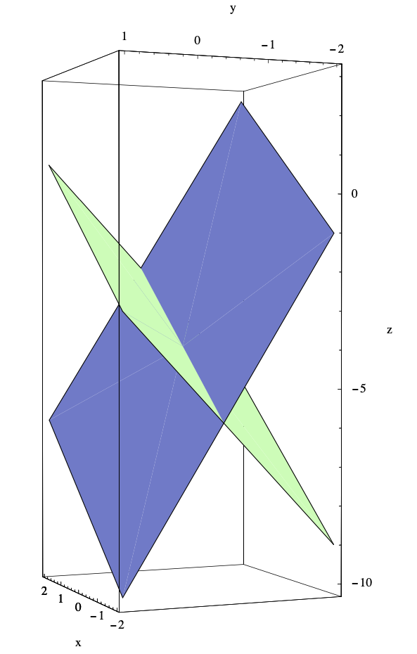
Example \(\PageIndex{14}\)

To find the angle θ between the two planes in \(\mathbb{R}^3\) with equations

\[ x+2 y-z=3 \nonumber \]

and

\[ x-3 y-z=5 , \nonumber \]

we first note that the corresponding normal vectors are \(\mathbf{m}=(1,2,-1)\) and \(\mathbf{n}=(1,-3,-1)\). Since \( \mathbf{m} \cdot \mathbf{n}=-4\), we will compute the angle between \(\mathbf{m}\) and \( - \mathbf{m}\). Hence

\[ \cos (\theta)=\frac{\mathbf{m} \cdot(-\mathbf{n})}{\|\mathbf{m}\|\|\mathbf{n}\|}=\frac{4}{\sqrt{6} \sqrt{11}}=\frac{4}{\sqrt{66}} . \nonumber \]

Thus, rounding to four decimal places,

\[ \theta=\cos ^{-1}\left(\frac{4}{\sqrt{66}}\right)=1.0560. \]

See Figure 1.4.11.

Figure \(\PageIndex{}\):\PageIndex{11}\): The planes \(x+2 y-z=3\) and \(x-3 y-z=5\)

Example \(\PageIndex{15}\)

The planes in \(\mathbb{R}^3\) with equations

\[ 3 x+y-2 z=3 \nonumber \]

and

\[ 6 x+2 y-4 z=13 \nonumber \]

are parallel since their normal vectors are \(\mathbf{m}=(3,1,-2)\) and \(\mathbf{n}=(6,2,-4)\) and \(\mathbf{n}=2 \mathbf{m} \).