1.5: Linear and Affine Functions
- Page ID
- 22922
One of the central themes of calculus is the approximation of nonlinear functions by linear functions, with the fundamental concept being the derivative of a function. This section will introduce the linear and affine functions which will be key to understanding derivatives in the chapters ahead.
Linear functions
In the following, we will use the notation \( f: \mathbb{R}^{m} \rightarrow \mathbb{R}^{n} \) to indicate a function whose domain is a subset of \(\mathbb{R}^{m}\) and whose range is a subset of \( \mathbb{R}^{n}\). In other words, \(f\) takes a vector with \(m\) coordinates for input and returns a vector with \(n\) coordinates. For example, the function
\[ f(x, y, z)=\left(\sin (x+y), 2 x^{2}+z\right) \nonumber \]
is a function from \( \mathbb{R}^{3}\) to \(\mathbb{R}^{2}\).
Definition \(\PageIndex{1}\)
We say a function \(L: \mathbb{R}^{m} \rightarrow \mathbb{R}^{m}\) is linear if (1) for any vectors \(\mathbf{x}\) and \(\mathbf{y}\) in \(\mathbb{R}^{m}\),
\[ L(\mathbf{x}+\mathbf{y})=L(\mathbf{x})+L(\mathbf{y}), \]
and (2) for any vector \(\mathbf{x}\) in \(\mathbb{R}^{m}\) and scalar \(a\),
\[ L(a \mathbf{x})=a L(\mathbf{x}). \]
Example \(\PageIndex{1}\)
Suppose \(f: \mathbb{R} \rightarrow \mathbb{R}\) is defined by \(f(x)=3 x\). Then for any \(x\) and \(y\) in \(\mathbb{R}\),
\[ f(x+y)=3(x+y)=3 x+3 y=f(x)+f(y), \nonumber \]
and for any scalar \(a\),
\[ f(a x)=3 a x=a f(x). \nonumber \]
Thus \(f\) is linear.
Example \(\PageIndex{2}\)
Suppose \(L: \mathbb{R}^{2} \rightarrow \mathbb{R}^{3}\) is defined by
\[ L\left(x_{1}, x_{2}\right)=\left(2 x_{1}+3 x_{2}, x_{1}-x_{2}, 4 x_{2}\right). \nonumber \]
Then if \(\mathbf{x}=\left(x_{1}, x_{2}\right)\) and \(\mathbf{y}=\left(y_{1}, y_{2}\right)\) are vectors in \(\mathbb{R}^2\),
\[ \begin{aligned}
L(\mathbf{x}+\mathbf{y}) &=L\left(x_{1}+y_{1}, x_{2}+y_{2}\right) \\
&=\left(2\left(x_{1}+y_{1}\right)+3\left(x_{2}+y_{2}\right), x_{1}+y_{1}-\left(x_{2}+y_{2}\right), 4\left(x_{2}+y_{2}\right)\right) \\
&=\left(2 x_{1}+3 x_{2}, x_{1}-x_{2}, 4 x_{2}\right)+\left(2 y_{1}+3 y_{2}, y_{1}-y_{2}, 4 y_{2}\right) \\
&=L\left(x_{1}, x_{2}\right)+L\left(y_{1}, y_{2}\right) \\
&=L(\mathbf{x})+L(\mathbf{y}).
\end{aligned}\]
Also, for \( \mathbf{x}=\left(x_{1}, x_{2}\right)\) and any scalar \(a\), we have
\[ \begin{aligned}
L(a \mathbf{x}) &=L\left(a x_{1}, a x_{2}\right) \\
&=\left(2 a x_{1}+3 a x_{2}, a x_{1}-a x_{2}, 4 a x_{2}\right) \\
&=a\left(2 x_{2}+3 x_{2}, x_{1}-x_{2}, 4 x_{2}\right) \\
&=a L(\mathbf{x}).
\end{aligned} \]
Thus \(L\) is linear.
Now suppose \( L: \mathbb{R} \rightarrow \mathbb{R}\) is a linear function and let \(a=L(1)\). Then for any real number \(x\),
\[ L(x)=L(1 x)=x L(1)=a x. \]
Since any function \(L: \mathbb{R} \rightarrow \mathbb{R}\) defined by \(L(x)=a x\), where \(a\) is a scalar, is linear (see Exercise 1), it follows that the only functions \( L: \mathbb{R} \rightarrow \mathbb{R}\) which are linear are those of the form \(L(x)=a x\) for some real number \(a\). For example, \(f(x)=5 x\) is a linear function, but \(g(x)=\sin (x) \) is not.
Next, suppose \(L: \mathbb{R}^{m} \rightarrow \mathbb{R}\) is linear and let \(a_{1}=L\left(\mathbf{e}_{1}\right), a_{2}=L\left(\mathbf{e}_{2}\right), \ldots, a_{m}=L\left(\mathbf{e}_{m}\right)\). If \(\mathbf{x}=\left(x_{1}, x_{2}, \ldots, x_{m}\right)\) is a vector in \(\mathbb{R}^{m}\), then we know that
\[ \mathbf{x}=x_{1} \mathbf{e}_{1}+x_{2} \mathbf{e}_{2}+\cdots+x_{m} \mathbf{e}_{m}. \nonumber \]
Thus
\begin{align}
L(\mathbf{x}) &=L\left(x_{1} \mathbf{e}_{1}+x_{2} \mathbf{e}_{2}+\cdots+x_{m} \mathbf{e}_{m}\right) \nonumber \\
&=L\left(x_{1} \mathbf{e}_{1}\right)+L\left(x_{2} \mathbf{e}_{2}\right)+\cdots+L\left(x_{m} \mathbf{e}_{m}\right) \nonumber\\
&=x_{1} L\left(\mathbf{e}_{1}\right)+x_{2} L\left(\mathbf{e}_{2}\right)+\cdots+x_{m} L\left(\mathbf{e}_{m}\right) \label{} \\
&=x_{1} a_{1}+x_{2} a_{2}+\cdots+x_{m} a_{m} \nonumber\\
&=\mathbf{a} \cdot \mathbf{x}, \nonumber
\end{align}
where \(a=\left(a_{1}, a_{2}, \ldots, a_{m}\right)\). Since for any vector \(\mathbf{a}\) in \(\mathbb{R}^m\), the function \(L(\mathbf{x})=\mathbf{a} \cdot \mathbf{x}\) is linear (see Exercise 1), it follows that the only functions \(L: \mathbb{R}^{m} \rightarrow \mathbb{R}\) which are linear are those of the form \(L(\mathbf{x})=\mathbf{a} \cdot \mathbf{x}\) for some fixed vector \(\mathbf{a}\) in \(\mathbb{R}^m\). For example,
\[ f(x, y)=(2,-3) \cdot(x, y)=2 x-3 y \nonumber\]
is a linear function from \(\mathbb{R}^2\) to \(R\), but
\[f(x, y, z)=x^{2} y+\sin (z) \nonumber \]
is not a linear function from \(\mathbb{R}^3\) to \(R\).
Now consider the general case where \(L: \mathbb{R}^{m} \rightarrow \mathbb{R}^{n}\) is a linear function. Given a vector \(\mathbf{x}\) in \(\mathbb{R}^{m}\), let \(L_{k}(\mathbf{x})\) be the \(k\)th coordinate of \(L(\mathbf{x}), k=1,2, \ldots, n\). That is,
\[L(\mathbf{x})=\left(L_{1}(\mathbf{x}), L_{2}(\mathbf{x}), \ldots, L_{n}(\mathbf{x})\right). \nonumber \]
Since \(L\) is linear, for any \(\mathbf{x}\) and \(\mathbf{y}\) in \(\mathbb{R}^m\) we have
\[ L(\mathbf{x}+\mathbf{y})=L(\mathbf{x})+L(\mathbf{y}), \nonumber \]
or, in terms of the coordinate functions,
\begin{aligned}
\left(L_{1}(\mathbf{x}+\mathbf{y}), L_{2}(\mathbf{x}+\mathbf{y}), \ldots, L_{n}(\mathbf{x}+\mathbf{y})\right)=\left(L_{1}(\mathbf{x}), L_{2}(\mathbf{x}), \ldots,\right.&\left.L_{n}(\mathbf{x})\right) \\
&+\left(L_{1}(\mathbf{y}), L_{2}(\mathbf{y}), \ldots, L_{n}(\mathbf{y})\right) \\
=\left(L_{1}(\mathbf{x})+L_{1}(\mathbf{y}), L_{2}\right.&(\mathbf{x})+L_{2}(\mathbf{y}) \\
&\left.\ldots, L_{n}(\mathbf{x})+L_{n}(\mathbf{y})\right).
\end{aligned}
Hence \(L_{k}(\mathbf{x}+\mathbf{y})=L_{k}(\mathbf{x})+L_{k}(\mathbf{y})\) for \(k=1,2, \ldots, n\). Similarly, if \(\mathbf{x}\) is in \(\mathbb{R}^{m}\) and \(a\) is a scalar, then \(L(a \mathbf{x})=a L(\mathbf{x})\), so
\begin{aligned}
\left(L_{1}(a \mathbf{x}), L_{2}(a \mathbf{x}), \ldots, L_{n}(a \mathbf{x})\right.&=a\left(L_{1}(\mathbf{x}), L_{2}(\mathbf{x}), \ldots, L_{n}(x)\right) \\
&=\left(a L_{1}(\mathbf{x}), a L_{2}(\mathbf{x}), \ldots, a L_{n}(x)\right) .
\end{aligned}
Hence \(L_{k}(a \mathbf{x})=a L_{k}(\mathbf{x})\) for \(k=1,2, \ldots, n\). Thus for each \(k=1,2, \ldots, n, L_{k}: \mathbb{R}^{m} \rightarrow \mathbb{R}\) is a linear function. It follows from our work above that, for each \(k=1,2, \ldots, n\), there is a fixed vector \(\mathbf{a}_{k}\) in \(\mathbb{R}^{m}\) such that \(L_{k}(x)=\mathbf{a}_{k} \cdot \mathbf{x}\) for all \(\mathbf{x}\) in \(\mathbb{R}^{m}\). Hence we have
\[L(\mathbf{x})=\left(\mathbf{a}_{1} \cdot \mathbf{x}, \mathbf{a}_{2} \cdot \mathbf{x}, \ldots, \mathbf{a}_{n} \cdot \mathbf{x}\right) \label{1.5.5} \]
for all \(\mathbf{x}\) in \(\mathbb{R}^m\). Since any function defined as in (\(\ref{1.5.5}\)) is linear (see Exercise 1 again), it follows that the only linear functions from \(\mathbb{R}^m\) to \(\mathbb{R}^n\) must be of this form.
Theorem \(\PageIndex{1}\)
If \(L: \mathbb{R}^{m} \rightarrow \mathbb{R}^{n}\) is linear, then there exist vectors \(\mathbf{a}_{1}, \mathbf{a}_{2}, \ldots, \mathbf{a}_{n}\) in \(\mathbb{R}^{m}\) such that
\[L(\mathbf{x})=\left(\mathbf{a}_{1} \cdot \mathbf{x}, \mathbf{a}_{2} \cdot \mathbf{x}, \ldots, \mathbf{a}_{n} \cdot \mathbf{x}\right) \label{1.5.6}\]
for all \(\mathbf{x}\) in \(\mathbb{R}^{m}\).
Example \(\PageIndex{3}\)
In a previous example, we showed that the function \(L: \mathbb{R}^{2} \rightarrow \mathbb{R}^{3}\) defined by
\[ L\left(x_{1}, x_{2}\right)=\left(2 x_{1}+3 x_{2}, x_{1}-x_{2}, 4 x_{2}\right) \nonumber \]
is linear. We can see this more easily now by noting that
\[ L\left(x_{1}, x_{2}\right)=\left((2,3) \cdot\left(x_{1}, x_{2}\right),(1,-1) \cdot\left(x_{1}, x_{2}\right),(0,4) \cdot\left(x_{1}, x_{2}\right)\right). \nonumber \]
Example \(\PageIndex{4}\)
The function
\[ f(x, y, z)=(x+y, \sin (x+y+z)) \nonumber \]
is not linear since it cannot be written in the form of (\(\ref{1.5.6}\)). In particular, the function \(f_{2}(x, y, z)=\sin (x+y+z)\) is not linear; from our work above, it follows that \(f\) is not linear.
Matrix Notation
We will now develop some notation to simplify working with expressions such as (\(\ref{1.5.6}\)). First, we define an \(n \times m\) matrix to be to be an array of real numbers with \(n\) rows and \(m\) columns. For example,
\[ M=\left[\begin{array}{rr}
2 & 3 \\
1 & -1 \\
0 & 4
\end{array}\right] \nonumber \]
is a \(3 \times 2\) matrix. Next, we will identify a vector \(\mathbf{x}=\left(x_{1}, x_{2}, \ldots, x_{m}\right)\) in \(\mathbb{R}^{m}\) with the \(m \times 1\) matrix
\[\mathbf{x}=\left[\begin{array}{c}
x_{1} \\
x_{2} \\
\vdots \\
x_{m}
\end{array}\right], \nonumber \]
which is called a column vector. Now define the product \(M \mathbf{x}\) of an \(n \times m\) matrix \(M\) with an \(m \times 1\) column vector \(\mathbf{x}\) to be the \(n \times 1\) column vector whose \(k\)th entry, \(k=1,2, \ldots, n\), is the dot product of the \(k\)th row of \(M\) with \(\mathbf{x}\). For example,
\[ \left[\begin{array}{rr}
2 & 3 \\
1 & -1 \\
0 & 4
\end{array}\right]\left[\begin{array}{l}
2 \\
1
\end{array}\right]=\left[\begin{array}{l}
4+3 \\
2-1 \\
0+4
\end{array}\right]=\left[\begin{array}{l}
7 \\
1 \\
4
\end{array}\right]. \nonumber \]
In fact, for any vector \(\mathbf{x}=\left(x_{1}, x_{2}\right)\) in \(\mathbb{R}^{2}\),
\[ \left[\begin{array}{rr}
2 & 3 \\
1 & -1 \\
0 & 4
\end{array}\right]\left[\begin{array}{l}
x_{1} \\
x_{2}
\end{array}\right]=\left[\begin{array}{c}
2 x_{1}+3 x_{2} \\
x_{1}-x_{2} \\
4 x_{2}
\end{array}\right]. \nonumber \]
In other words, if we let
\[ L\left(x_{1}, x_{2}\right)=\left(2 x_{1}+3 x_{2}, x_{1}-x_{2}, 4 x_{2}\right), \nonumber \]
as in a previous example, then, using column vectors, we could write
\[ L\left(x_{1}, x_{2}\right)=\left[\begin{array}{cc}
2 & 3 \\
1 & -1 \\
0 & 4
\end{array}\right]\left[\begin{array}{l}
x_{1} \\
x_{2}
\end{array}\right]. \nonumber \]
In general, consider a linear function \(L: \mathbb{R}^{m} \rightarrow \mathbb{R}^{n}\) defined by
\[ L(\mathbf{x})=\left(\mathbf{a}_{1} \cdot \mathbf{x}, \mathbf{a}_{2} \cdot \mathbf{x}, \ldots, \mathbf{a}_{n} \cdot \mathbf{x}\right) \]
for some vectors \(\mathbf{a}_{1}, \mathbf{a}_{2}, \ldots, \mathbf{a}_{n}\) in \(\mathbb{R}^{m}\). If we let \(M\) be the \(n \times m\) matrix whose \(k\)th row is \(\mathbf{a}_{k}, k=1,2, \ldots, n\), then
\[ L(\mathbf{x})=M \mathbf{x} \]
for any \(\mathbf{x}\) in \(\mathbb{R}^m\). Now, from our work above,
\[ \mathbf{a}_{k}=\left(L_{k}\left(\mathbf{e}_{1}\right), L_{k}\left(\mathbf{e}_{2}\right), \ldots, L_{k}\left(\mathbf{e}_{m}\right)\right. ,\]
which means that the \(j\)th column of \(M\) is
\[ \left[\begin{array}{c}
L_{1}\left(\mathbf{e}_{j}\right) \\
L_{2}\left(\mathbf{e}_{j}\right) \\
\vdots \\
L_{n}\left(\mathbf{e}_{j}\right)
\end{array}\right], \label{1.5.10} \]
\(j=1,2, \ldots, m\). But (\(\ref{1.5.10}\)) is just \(L\left(\mathbf{e}_{j}\right)\) written as a column vector. Hence \(M\) is the matrix whose columns are given by the column vectors \(L\left(\mathbf{e}_{1}\right), L\left(\mathbf{e}_{2}\right), \ldots, L\left(\mathbf{e}_{m}\right)\).
Theorem \(\PageIndex{2}\)
Suppose \(L: \mathbb{R}^{m} \rightarrow \mathbb{R}^{n}\) is a linear function and \(M\) is the \(n \times m\) matrix whose \(j\)th column is \(L\left(\mathbf{e}_{j}\right), j=1,2, \ldots, m\). Then for any vector \(\mathbf{x}\) in \(\mathbb{R}^m\),
\[ L(\mathbf{x})=M \mathbf{x}. \]
Example \(\PageIndex{5}\)
Suppose \(L: \mathbb{R}^{3} \rightarrow \mathbb{R}^{2}\) is defined by
\[ L(x, y, z)=(3 x-2 y+z, 4 x+y). \nonumber \]
Then
\[ \begin{aligned}
&L\left(\mathbf{e}_{1}\right)=L(1,0,0)=(3,4), \\
&L\left(\mathbf{e}_{2}\right)=L(0,1,0)=(-2,1),
\end{aligned} \]
and
\[ L\left(\mathbf{e}_{3}\right)=L(0,0,1)=(1,0). \nonumber \]
So if we let
\[ M=\left[\begin{array}{rrr}
3 & -2 & 1 \nonumber \\
4 & 1 & 0
\end{array}\right], \nonumber \]
then
\[ L(x, y, z)=\left[\begin{array}{lrl}
3 & -2 & 1 \\
4 & 1 & 0
\end{array}\right]\left[\begin{array}{l}
x \\
y \\
z
\end{array}\right]. \nonumber \]
For example,
\[ \begin{equation}
L(1,-1,3)=\left[\begin{array}{rrr}
3 & -2 & 1 \\
4 & 1 & 0
\end{array}\right]\left[\begin{array}{r}
1 \\
-1 \\
3
\end{array}\right]=\left[\begin{array}{l}
3+2+3 \\
4-1+0
\end{array}\right]=\left[\begin{array}{l}
8 \\
3
\end{array}\right].
\end{equation} \nonumber \]
Example \(\PageIndex{6}\)
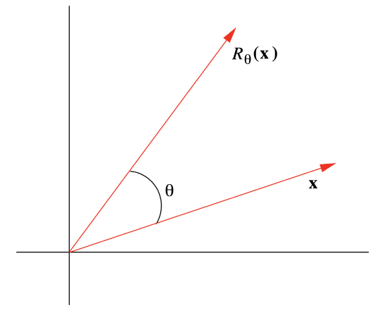
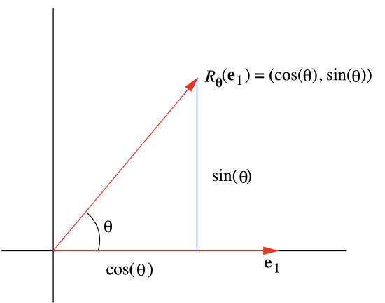
Let \(\begin{equation} R_{\theta}: \mathbb{R}^{2} \rightarrow \mathbb{R}^{2} \end{equation}\) be the function that rotates a vector \(\mathbf{x}\) in \(\mathbb{R}^2\) counterclockwise through an angle θ, as shown in Figure 1.5.1. Geometrically, it seems reasonable that \(R_\theta\) is a linear function; that is, rotating the vector \(\mathbf{x}+\mathbf{y} \) through an angle θ should give the same result as first rotating \(\mathbf{x}\) and \(\mathbf{y}\) separately through an angle θ and then adding, and rotating a vector \(a \mathbf{x}\) through an angle θ should give the same result as first rotating \( \mathbf{x}\) through an angle θ and then multiplying by \(a\). Now, from the definition of \(\cos(\theta)\) and \(\sin(\theta)\),
\[ R_{\theta}\left(\mathbf{e}_{1}\right)=R_{\theta}(1,0)=(\cos (\theta), \sin (\theta)) \nonumber \]
(see Figure 1.5.2), and, since \(\mathbf{e}_{2}\) is \(\mathbf{e}_{1}\) rotated, counterclockwise, through an angle \(\frac{\pi}{2}\),
\[ R_{\theta}\left(\mathbf{e}_{2}\right)=R_{\theta+\frac{\pi}{2}}\left(\mathbf{e}_{1}\right)=\left(\cos \left(\theta+\frac{\pi}{2}\right), \sin \left(\theta+\frac{\pi}{2}\right)\right)=(-\sin (\theta), \cos (\theta)). \nonumber \]
\[ R_{\theta}(x, y)=\left[\begin{array}{rr}
\cos (\theta) & -\sin (\theta) \\
\sin (\theta) & \cos (\theta)
\end{array}\right]\left[\begin{array}{l}
x \\
y
\end{array}\right]. \label{1.5.12} \]


You are asked in Exercise 9 to verify that the linear function defined in (\(\ref{1.5.12}\)) does in fact rotate vectors through an angle θ in the counterclockwise direction. Note that, for example, when \(\theta=\frac{\pi}{2}\), we have
\[ R_{\frac{\pi}{2}}(x, y)=\left[\begin{array}{rr}
0 & -1 \\
1 & 0
\end{array}\right]\left[\begin{array}{l}
x \\
y
\end{array}\right]. \nonumber \]
In particular, note that \(R_{\frac{\pi}{2}}(1,0)=(0,1)\) and \(R_{\frac{\pi}{2}}(0,1)=(-1,0)\); that is, \(R_{\frac{\pi}{2}}\) takes \(\mathbf{e}_{1}\) to \(\mathbf{e}_{2}\) and \(\mathbf{e}_{2}\) to \(-\mathbf{e}_{1}\). For another example, if \(\theta=\frac{\pi}{6}\), then
\[ R_{\frac{\pi}{6}}(x, y)=\left[\begin{array}{cc}
\frac{\sqrt{3}}{2} & -\frac{1}{2} \\
\frac{1}{2} & \frac{\sqrt{3}}{2}
\end{array}\right]\left[\begin{array}{l}
x \\
y
\end{array}\right]. \nonumber \]
In particular,
\[ \begin{equation}
R_{\frac{\pi}{6}}(1,2)=\left[\begin{array}{cc}
\frac{\sqrt{3}}{2} & -\frac{1}{2} \\
\frac{1}{2} & \frac{\sqrt{3}}{2}
\end{array}\right]\left[\begin{array}{l}
1 \\
2
\end{array}\right]=\left[\begin{array}{c}
\frac{\sqrt{3}}{2}-1 \\
\frac{1}{2}+\sqrt{3}
\end{array}\right]=\left[\begin{array}{c}
\frac{\sqrt{3}-2}{2} \\
\frac{1+2 \sqrt{3}}{2}
\end{array}\right]
\end{equation}. \nonumber \]
Affine functions
Definition \(\PageIndex{2}\)
We say a function \(A: \mathbb{R}^{m} \rightarrow \mathbb{R}^{n}\) is affine if there is a linear function \(L : \mathbb{R}^{m} \rightarrow \mathbb{R}^{n} \) and a vector \(\mathbf{b}\) in \(\mathbb{R}^n\) such that
\[ A(\mathbf{x})=L(\mathbf{x})+\mathbf{b}\]
for all \(\mathbf{x}\) in \( \mathbb{R}^m\).
An affine function is just a linear function plus a translation. From our knowledge of linear functions, it follows that if \(A: \mathbb{R}^{m} \rightarrow \mathbb{R}^{n}\) is affine, then there is an \(n \times m\) matrix \(M\) and a vector \(\mathbf{b}\) in \(\mathbb{R}^n\) such that
\[ A(\mathbf{x})=M \mathbf{x}+\mathbf{b}\]
for all \(\mathbf{x}\) in \(\mathbb{R}^m\). In particular, if \(f: \mathbb{R} \rightarrow \mathbb{R}\) is affine, then there are real numbers \(m\) and \(b\) such that
\[ f(x)=m x+b\]
for all real numbers \(x\).
Example \(\PageIndex{7}\)
The function
\[A(x, y)=(2 x+3, y-4 x+1) \nonumber \]
is an affine function from \(\mathbb{R}^{2}\) to \(\mathbb{R}^{2}\) since we may write it in the form
\[ A(x, y)=L(x, y)+(3,1), \nonumber \]
where \(L\) is the linear function
\[ L(x, y)=(2 x, y-4 x). \nonumber \]
Note that \(L(1,0)=(2,-4)\) and \(L(0,1)=(0,1)\), so we may also write \(A\) in the form
\[A(x, y)=\left[\begin{array}{rr}
2 & 0 \\
-4 & 1
\end{array}\right]\left[\begin{array}{l}
x \\
y
\end{array}\right]+\left[\begin{array}{l}
3 \\
1
\end{array}\right] . \nonumber \]
Example \(\PageIndex{8}\)
The affine function
\[A(x, y)=\left[\begin{array}{cc}
\frac{1}{\sqrt{2}} & -\frac{1}{\sqrt{2}} \\
\frac{1}{\sqrt{2}} & \frac{1}{\sqrt{2}}
\end{array}\right]\left[\begin{array}{l}
x \\
y
\end{array}\right]+\left[\begin{array}{l}
1 \\
2
\end{array}\right] \nonumber \]
first rotates a vector, counterclockwise, in \(\mathbb{R}^{2}\) through an angle of \(\frac{\pi}{4}\) and then translates it by the vector \( (1,2) \).


