1.5: Congruences

In this section we shall develop some aspects of the theory of divisibility and congruences.

If

\(a = \prod p^{\alpha}\) and \(b = \prod p^{\beta}\)

then it is easily seen that

\((a, b) = \prod p^{\text{min}(\alpha, \beta)}\) while \([a, b] = \prod p^{\text{max} (\alpha, \beta)}.\)

From these it follows easily that \((a, b) \cdot [a, b] = a \cdot b\). We leave it as an exercise to show that

\((a, b) = \dfrac{1}{a} \sum_{a = 1}^{a - 1} \sum_{\beta = 1}^{a - 1} e^{2\pi i \dfrac{b}{a} \alpha \beta}.\)

The notation \(a \equiv b\) (mod \(m\)) for \(m\ |\ (a - b)\) is due to Gauss. Rather obvious properties of this congruence are \(a \equiv a\), \(a \equiv b \Rightarrow b \equiv a\), and \(a \equiv b\) and \(b \equiv c \Rightarrow a \equiv c\), i.e., \(\equiv\) is an equivalence relation. It is also easily proved that \(a \equiv b\) and \(c \equiv d\) together imply \(ac \equiv bd\); in particular \(a \equiv b \Rightarrow ka \equiv kb\). However the converse is not true in general. Thus \(2 \times 3 = 4 \times 3\) (mod 6) does not imply \(2 \equiv 4\) (mod 6). However, if \((k, m) = 1\) than \(ka \equiv kb\) does imply \(a \equiv b\).

Another important result is the following.

Theorem

If \(a_1, a_2, ..., a_{\varphi(m)}\) form a complete residue system mod \(m\) then so does \(aa_1\), \(aa_2\), ..., \(aa_{\varphi(m)}\) provided \((a, m) = 1\).

Proof

We have \(\varphi(m)\) residues. If two of them are congruent \(aa_i \equiv aa_j\), \(a(a_i - a_j) \equiv 0\). But \((a, m) = 1\) so that \(a_i \equiv a_j\).

An application of these ideas is to the important Euler’s theorem:

Theorem

If \((a, m) = 1\) then \(a^{\varphi(m)} \equiv 1\) (mod \(m\)).

Proof

Since \(a_1, a_2, ..., a_{\varphi(m)}\) are congruent to \(aa_1\), \(aa_2\), ..., \(aa_{\varphi(m)}\) insome order, their products are congruent. Hence

\(a^{\varphi(m)} a_1 a_2 \cdot\cdot\cdot a_{\varphi(m)} \equiv a_1 a_2 \cdot\cdot\cdot a_{\varphi(m)}\)

and the result follows.

A special case of primary importance is the case \(m = p\) where we have

\((a, p) = 1 \Longrightarrow a^{p - 1} \equiv 1\) (mod \(p\))

Multiplying by \(a\) we have for all cases \(a^p \equiv a\) (mod \(p\)). Another proof of this result goes by induction on \(a\); we have

\((a + 1)^p = a^p + {p \choose 1} a^{p - 1} + \cdot\cdot\cdot + 1 \equiv a^p \equiv a\) (mod \(p\))

One could also use the multinomial theorem and consider \((1 + 1 + \cdot\cdot\cdot + 1)^p\).

Still another proof goes by considering the number of regular convex \(p\)-gons where each edge can be colored in one of a colors. The number of such polygons is \(a^p\), of which a are monochromatic. Hence \(a^p − a\) are not monochromatic and these come in sets of \(p\) each by rotation through \(\dfrac{2\pi n}{p}, n = 1,2, ..., p−1\). The idea behind this proof has considerable applicability and we shall return to at least one other application a little later. We also leave as an exercise the task of finding a similar proof of Euler’s theorem.

The theorems of Fermat and Euler may also be conveniently viewed from a group-theoretic viewpoint. The integers relatively prime to \(m\) and \(< m\) form a group under multiplication mod \(m\). The main thing to check here is that every element has an inverse in the system. If we seek an inverse for a we form \(aa_1, aa_2, ..., aa_{\varphi(m)}\). We have already seen that these are \(\varphi(m)\) numbers incongruent mod \(m\) and relatively prime to \(m\). Thus one of them must be the unit and the result follows.

We now regain Euler’s proof from that of Lagrange’s which states that if \(a\) is an element of a group \(G\) of order \(m\), then \(a^m = 1\). In our case this means \(a^{\varphi(m)} \equiv 1\) or \(a^{p−1} \equiv 1\) if \(p\) is a prime.

The integers under \(p\) form a field with respect to + and \(\times\). Many of the important results of number theory are based on the fact that the multiplicative part of this group (containing \(p − 1\) elements) is cyclic, i.e., there exists a number \(g\) (called primitive root of \(p\)) such that \(1 = g^0, g^10,g^2, ... , g^{p−1}\) are incongruent mod \(p\). This fact is not trivial but we omit the proof. A more general group-theoretic result in which it is contained states that every finite field is automatically Abelian and its multiplicative group is cyclic.

In the ring of polynomials with coefficients in a field many of the theorems of elementary theory of equations holds. For example if \(f(x)\) is a polynomial whose elements are residue classes mod \(p\) then \(f(x) \equiv 0\) (mod \(p\)) has at most \(p\) solutions. Further if \(r\) is a root then \(x − r\) is a factor. On the other hand, it is not true that \(f(x) \equiv 0\) (mod \(p\)) has at least one root.

Since \(x^p − x \equiv 0\) has at most \(p\) roots we have the factorization

\(x^p - x \equiv x(x - 1)(x - 2) \cdot\cdot\cdot (x - p + 1)\) (mod \(p\))

Comparing coefficients of \(x\) we have \((p - 1)! \equiv -1\) (mod \(p\)) which is Wilson's theorem.

Cayley gave a geometrical proof of Wilson’s theorem as follows. Consider the number of directed p-gons with vertices of a regular p-gon. (See Figure 3.)

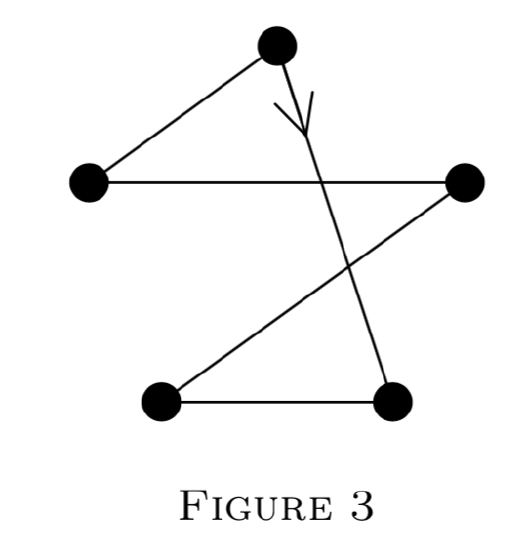
There are \((p - 1)!\) in number of which \(p - 1\) are regular. Hence the nonregular ones are \((p - 1)! - (p - 1)\) in number and these come in sets of \(p\) by rotation. Hence

\((p - 1)! - (p - 1) \equiv 0\) (mod \(p\))

and

\((p - 1)! + 1 \equiv 0\) (mod \(p\))

follows.

One can also give a geometrical proof which simultaneously yields both

Fermat’s and Wilson’s theorems and we suggest as a problem finding such a proof.

Wilson’s theorem yields a necessary and sufficient condition for primality: \(p\) is prime if and only if \((p − 1)! \equiv −1\), but this is hardly a practical criterion.

Congruences with Given Roots

Let \(a_1\), \(a_2\), ..., \(a_k\) be a set of distinct residue classes (mod \(n\)). If there exists a polynomial with integer coefficients such that \(f(x) \equiv 0\) (mod \(m\)) has roots \(a_1\), \(a_2\), ..., \(a_k\) and no others, we call this set compatible (mod \(n\)). Let the number of compatible sets (mod \(n\)) be denoted by \(C(n)\). Since the number of subsets of the set consisting of 0, 1, 2, ..., \(n - 1\) is \(2^n\), we call \(c(n) = \dfrac{C(n)}{2^n}\) the coefficient of comatiblity of \(n\).

If \(n = p\) is a prime then the congruence

\((x - a_1) (x - a_2) \cdot\cdot\cdot (x - a_k) \equiv 0\) (mod \(n\))

has precisely the roots \(a_1, a_2, ..., a_n\). Hence \(c(p) = 1\). In a recent paper M. M. Chokjnsacka Pnieswaka has shown that \(c(4) = 1\) while \(c(n) < 1\) for \(n = 6, 8, 9, 10\). We shall prove that \(c(n) < 1\) for every composite \(n \ne 4\). We can also prove that the average value of \(c(n)\) is zero, i.e.,

\(\text{lim}_{n \to \infty} \dfrac{1}{n} (c(1) + c(2) + \cdot\cdot\cdot c(n)) = 0\)

Since \(c(n) = 1\) for \(n = 1\) and \(n = p\) we consider only the case where \(n\) is composite. Suppose then that the unique prime factorization of \(n\) is given by \(p_{1}^{\alpha_1} p_{2}^{\alpha_2} \cdot\cdot\cdot\) with

\(p_{1}^{\alpha_1} > p_{2}^{\alpha_2} > \cdot\cdot\cdot\)

Consider separately the cases

(1) \(n\) has more than one prime divisor, and

(2) \(n = p^{\alpha}, \alpha > 1\).

In case (1) we can write

\(n = a \cdot b\), \((a, b) = 1, a > b > 1.\)

We now show that if \(f(a) \equiv f(b) \equiv 0\) then \(f(0) \equiv 0\).

Proof. Let \(f(x) = c_0 + c_1 + \cdot\cdot\cdot + c_m x^m\). Then

\(0 \equiv af(b) \equiv ac_0\) (mod \(n\)) and

\(0 \equiv bf(a) \equiv bc_0\) (mod \(n\)).

Now since \((a, b) = 1\) there exist \(r\), \(s\), such that \(ar + bs = 1\) so that \(c_0 (ar + bs) \equiv 0\) and \(c_0 \equiv 0\).

In case (2) we can write

\(n = p^{\alpha - 1} p.\)

We show that \(f(p^{\alpha - 1}) \equiv 0\) and \(f(0) \equiv 0\) imply \(f(kp^{\alpha - 1} \equiv 0\), \(k = 2, 3, ... .\)

Proof. Since \(f(0) \equiv 0\), we have \(c_0 \equiv 0\),

\(f(x) \equiv c_1 + c_2 x^2 + \cdot\cdot\cdot + c_m x^m\), and

\(f(p^{\alpha - 1}) \equiv c_1 p^{\alpha - 1} \equiv 0\) (mod \(p^{\alpha}\)),

so that \(c_1 \equiv 0\) (mod \(p\)). But now \(f(kp^{\alpha - 1} \equiv 0\), as required.

On Relatively Prime Sequences Formed by Interating Polynomials (Lambek and Moser)

Bellman has recently posed the following problem. If \(p(x)\) is an irreducible polynomial with integer coefficients and \(p(x) > x\) for \(x > c\), prove that {\(p^n (c)\)} cannot be prime for all large \(n\). We do not propose to solve this problem but wish to make some remarks.

If \(p(x)\) is a polynomial with integer coeffcients, then so is the \(k^{\text{th}}\) iterate defined recursively by \(p^0 (x) = x\), \(p^{p + 1} (x) = p(p^k (x))\). If \(a\) and \(b\) are integers then

\[p^k (a) \equiv p^k (b)\ \ \ \ (\text{mod }(a - b))\]

In particular for \(a = p^n (c)\) and \(b = 0\) we have \(p^{k + n} (c) \equiv p^k (0)\) (mod \(p^n(c)\)).

Hence

\[(p^{k + n} (c), p^n (c)) = (p^k(0), p^n(c)).\]

We shall call a sequence {\(a_n\)}, \(n \ge 0\), relatively prime if \((a_m, a_n) = 1\) for all values of \(m, n\), with \(m \ne n\). From 5.2 we obtain

Theorem 1

{\(p^n (c)\)}, \(n \ge 0\), is relatively prime if and only if \((p^k(0), p^n(c)) = 1\) for all \(k \ge 0\), \(n \ge 0\)

From the follows immediately a result of Bellman: If \(p^k(0) = p(0) \ne 1\) for \(k \ge 1\) and if \((a, p(0)) = 1\) implies \((p(a), p(0)) = 1\) then {\(p^n(a)\)}, \(n \ge a\) is relatively prime whenever \((c, p(0)) = 1\).

We shall now construct all polynomials \(p(x)\) for which {\(p^n(c)\)}, \(n \ge 0\), is relatively prime for all \(c\). According to Theorem 1, \({p^k(0)} = \pm 1\) for all \(k \ge 1\), as if easily seen by taking \(n = k\) and \(c = 0\). But then {\(p^k(0)\)} must be one of the following six sequences:

1, 1, 1, ...

1, -1, 1, ...

1, -1, -1, ...

-1, 1, 1, ...

-1, 1, -1, ...

-1, -1, 1, ...

it is easily seen that the general solution of \(p(x)\) (with integer coefficients) of \(m\) equtions

\(p(a_k) = a_{k +1}\), \(k = 0, 1, 2, ..., m - 1.\)

is obtained from a particular solution \(p_1 (x)\) as follows.

\[p(x) = p_1 (x) + (x - a_1) (x - a_2) \cdot\cdot\cdot (x - a_{k - 1}) \cdot Q(x),\]\

where \(Q(x)\) is any polynomial with integer coefficients.

Theorem 2

{\(p^n (c)\)}, \(n \ge 0\), is relatively prime for all \(c\) if and only if \(p(x)\) belongs to one of the following six classes of polynomials.

\(1 + x (x - 1) \cdot Q(x)\)

\(1 - x - x^2 + x(x^2 - 1) \cdot Q(x)\)

\(1 - 2x^2 + x(x^2 - 1) \cdot Q(x)\)

\(2x^2 - 1 + x(x^2 - 1) \cdot Q(x)\)

\(x^2 - x - 1 + x(x^2 - 1) \cdot Q(x)\)

\(-1 + x(x + 1) \cdot Q(x)\)

Proof

In view of (5.3) we need only verify that the particular solutions yield the six sequences given above.

On the Distribution of Quadratic Residues

A large segment of number theory can be characterized by considering it to be the study of the first digit on the right of integers. Thus, a number is divisible by \(n\) if its first digit is zero when the number is expressed in base \(n\). Two numbers are congruent (mod \(n\)) if their first digits are the same in base \(n\). The theory of quadratic residues is concerned with the first digits of the squares. Of particular interest is the case where the base is a prime, and we shall restrict ourselves to this case.

If one takes for example \(p = 7\), then with congruences (mod 7) we have \(1^2 \equiv 1 \equiv 6^2\), \(2^2 \equiv 4 \equiv 5^2\), and \(3^2 \equiv 2 \equiv 4^2\); obviously, \(0^2 \equiv 0\). Thus 1, 2, 4 are squares and 3, 5, 6 are nonsquares or nonresidues. If \(a\) is a residue of \(p\) we write

\((\dfrac{a}{p}) = + 1\)

while if \(a\) is a nonresidue we write

\((\dfrac{a}{p}) = - 1\)

For \(p\ |\ c\) we write \((\dfrac{c}{p}) = 0\). This notation is due to Legendre. For \(p = 7\) the sequence \((\dfrac{a}{p})\) is thus

+ + - + - -.

For \(p = 23\) it turns out to be

+ + + + - + - + + - - + + - - + - + - - - -.

The situation is clarified if we again adopt the group theoretic point of view. The residue classes (mod \(p\)) form a field, whose multiplicative group (containing \(p − 1\) elements) is cyclic. If \(g\) is a generator of this group then the elements may be written \(g^1, g^2, ..., g^{p−1} = 1\). The even powers of \(g\) are the quadratic residues; they form a subgroup of index two. The odd powers of \(g\) are the quadratic nonresidues. From this point of view it is clear

res \(\times\) res = res, res \(\times\) nonres = nonres, nonres \(\times\) nonres = res.

Further 1/\(a\) represents the unique inverse of \(a\) (mod \(p\)) and will be a residue or nonresidue according as a itself is a residue or nonresidue.

The central theorem in the theory of quadratic residues and indeed one of the most central results of number theory is the Law of Quadratic Reciprocity first proved by Gauss about 1800. It states that

It leads to an algorithm for deciding the value of \((\dfrac{p}{q})\).

Over 50 proofs of this law have been given including recent proofs by Zassen-haus and by Lehmer. In Gauss’ first proof (he gave seven) he made use of the following lemma—which he tells us he was only able to prove with considerable difficulty. For \(p = 1\) (mod 4) the least nonresidue of \(p\) does not exceed \(2\sqrt{p}+1\). The results we want to discuss today are in part improvements of this result and more generally are concerned with the distribution of the sequence of + and − ’s in \((\dfrac{a}{p})\), \(a = 1, 2, ..., p − 1\).

In 1839 Dirichlet, as a by-product of his investigation of the class number of quadratic forms, established the following theorem: If \(p \equiv 3\) (mod 4) then among the integers \(1, 2, ..., \dfrac{p−1}{2}\), there are more residues than nonresidues. Though this is an elementary statement about integers, all published proofs, including recent ones given by Chung, Chowla, Whitman, Carlitz, and Moser involve Fourier series. Landau was quite anxious to have an elementary proof. Though somewhat related results have been given by Whitman and by Carlitz, Dirichlet’s result is quite isolated. Thus, no similar nontrivial result is known for other ranges.

In 1896 Aladow, in 1898 von Sterneck, and in 1906 Jacobsthall, took up the question of how many times the combinations ++, +−, −+, and −−appear. They showed that each of the four possibilities appeared, as one might expect, with frequency 1/4. In 1951 Perron examined the question again and proved that similar results hold if, instead of consecutive integers, one considers integers separated by a distance \(d\). J. B. Kelly recently proved a result that, roughly speaking, shows that the residues and non residues are characterized by this property. Jacobsthall also obtained partial results for the cases of 3 consecutive residues and non residues. Let \(R_n\) and \(N_n\) be the number of blocks of \(n\) consecutive residues and non residues respectively. One might conjecture that \(R_n \thicksim N_n \thicksim \dfrac{p}{2^n}\). Among those who contributed to this question are Vandiver, Bennet, Dorge, Hopf, Davenport, and A. Brauer. Perhaps the most interesting result is that of A. Brauer. He showed that for \(p > p_0 (n)\), \(R_n > 0\) and \(N_n > 0\). We shall sketch part of his proof. It depends on a very interesting result of Van der Waerden (1927). Given \(k\), \(\ell\), there exists an integer \(N = N(k, \ell)\) such that if one separates the integers \(1, 2, ..., N\) into \(k\) classes in any manner whatsoever, at least one of the classes will contain an arithmetic progression of length l. There are a number of unanswered questions about this theorem to which we shall return in a later section.

Returning to Brauer’s work, we shall show he proves that all large primes have, say, 7 consecutive residues. One separates the numbers \(1, 2, ..., p − 1\) into 2 classes, residues and nonresidues. If \(p\) is large enough one of these classes will contain, by Van der Waerden’s theorem, 49 terms in arithmetic progression, say

\(a, a + b, a + 2b, ..., a + 48b.\)

Now if \(\dfrac{a}{b} = c\) then we have 49 consecutive numbers of the same quadratic character, namely

\(c, c + 1, c + 2, ..., c + 48.\)

and the result is complete.

The proof of the existence of nonresidues is considerably more complicated. Furthermore it is interesting to note that the existence of block s like + − + − \(\cdot\cdot\cdot\) is not covered by these methods.

We now return to the question raised by Gauss. What can be said about the least nonresidue \(n_p\) of a prime? Since 1 is a residue, the corresponding question about residues is “what is the smallest prime residue \(r_p\) of \(p\)?”. These questions were attacked in the 1920s by a number of mathematicians including Nagel, Schur, Polya, Zeitz, Landau, Vandiver, Brauer, and Vinogradov. Nagel, for example, proved that for \(p \ne 7\), 23, \(n_p < \sqrt{p}\). Polya and Schur proved that

\(\sum_{n = a}^{b} (\dfrac{n}{p}) < \sqrt{p} \log p.\)

This implies that there are never more than \(\sqrt{p} \log p\) consecutive residues or nonresidues and that ranges much larger than \(\sqrt{p} \log p\) have about as many residues as nonresidues. Using this result and some theorems on the distribu- tion of primes, Vinogradov proved that for \(p > p_0\),

\(n_p < p^{\dfrac{1}{2\sqrt{e}}} \log ^2 p < n^{.303}.\)

Checking through Vinogradov's proof we found that by his method the \(p_0\) is excessively large, say \(p_0 > 10^{10^{10}}\). Nevertheless, in spite of numerous attempts this result of Vinogradov has not been much improved.

In 1938 Erd\(\ddot{o}\)s and Ko showed that the existence of small nonresidues was intimately connected with the nonexistence of the Euclidean Algorithm in quadratic fields. This led Brauer, Hua, Min to re-examine the question of explicit bounds for the least nonresidue. Brauer already in 1928 had proved a number of such results, typical of which is that for all \(p \equiv 1\) (mod 8),

\(n_p < (2p)^{.4} + 3 (2p)^{.2} + 1\)

and Hua and Min proved, for example, that for \(p > e^{250}\),

\(n_p < (60 \sqrt{p})^{.625}\).

Small primes (under 10,000,000) were considered by Bennet, Chatland, Brauer, Moser, and others.

Quite recently, the unproved extended Riemann hypothesis has been applied to these problems by Linnik, Chowla, Erd\(\ddot{o}\)s, and Ankeny. Thus, for example, Ankeny used the extended Riemann hypothesis to prove that \(n_p \ne O(\log ^2 p)\). In the opposite direction Pillai (1945) proved that \(p \ne o(\log \log p)\). Using first the Riemann hypothesis, and later some deep results of Linnik on primes in arithmetic progression, Friedlander and Chowla improved this to \(n_p \ne o(\log p)\).

Quite recently there have been a number of results in a somewhat different direction by Brauer, Nagel, Skolem, Redei, and Kanold. Redei’s method is particularly interesting. He uses a finite projective geometrical analogue of the fundamental theorem of Minkowski on con√vex bodies to prove that for \(p \equiv 1\) (mod 4), at least \(\dfrac{1}{7}\) of the numbers up to \(\sqrt{p}\) are residues and at least 1 are non residues. Our own recent contributions to the theory are along these lines. We shall outline some of this work.

Consider first the lattice of points in a square of side \(m\). We seek an estimate for \(V(m)\), the number of visible lattice points in the square. As on the previous paragraph we find

\([m]^2 = V(m) + V(\dfrac{m}{2}) + \cdot\cdot\cdot\)

and inverting by the Mobius inversion formula yields

\(V(m) = \sum_{d \ge 1} \mu (d) [\dfrac{m}{d}]^2\).

As before this leads to the asymptotic estimate

\(V(m) \thicksim \dfrac{6}{\pi^2} m^2.\)

We can however obtain explicit estimates for \(v(m)\) also. Indeed, from the exact formula for \(V(m)\) above one can show that for all \(m\), \(V (m) > .6m^2\). We now take \(m = [\sqrt{p}]\). For reasonably large \(p\) we shall have \(V([\sqrt{p}]) > .59m^2\). Now with each visible lattice point \((a, b)\) we associate the number \(\dfrac{a}{b}\) (mod \(p\)). We now show that distinct visible points correspond to distinct numbers. Thus if \(\dfrac{a}{b} = \dfrac{c}{d}\) then \(ad \equiv bc\). But \(ad < p\) and \(bc < p\). Hence \(ad = bc\) and \(\dfrac{a}{b} = \dfrac{c}{d}\). However \((a, b) = (c, d) = 1\) so that \(a = c\) and \(b = d\).

Since we have at least .59 distinct numbers represented by fractions \(\dfrac{a}{b}\), \(a < \sqrt{p}\), \(b < \sqrt{p}\), at least .09 of these will correspond to nonresidues. If \(R\) denotes the number of residues \(< \sqrt{p}\) and \(N\) the number of nonresidues \(< \sqrt{p}\), then \(R + N = \sqrt{p}\) and \(2RN > .09p\). Solving these inequalities gives \(R, N > .04 \sqrt{p}\). This is weaker than Nagel's result but has the advantage of holding for primes \(p \equiv 3\) (mod 4) as well as \(p \equiv 1\) (mod 4). Thus, exceptions turn out to be only the primes 7 and 23. For primes \(p \equiv 1\) (mod 4), −1 is a nonresidue and this can be used together with above method to get stronger results. One can also use the existence of many nonresidues < \(\sqrt{p}\) to prove the existence of one small nonresidue, but the results obtainable in this way are not as strong as Vinogradov’s result.