
10.1: Basics

- Last updated
- Feb 18, 2022
- Save as PDF

( \newcommand{\kernel}{\mathrm{null}\,}\)
10.1.1: Terminology and basic concepts
a rule which assigns to each input element from a set A a single output element from a set B
the set of all possible input elements for a function
a set containing all possible output elements for a function
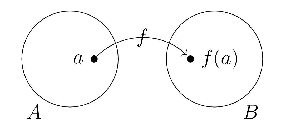
f is a function with domain A and codomain B
the process/algorithm/rule/formula that describes how each input element from the domain will be transformed into an output element in the codomain
function f:A→B associates the codomain element b∈B to the domain element a∈A
alternative notation for f(a)=b
when f(a)=b we say that b is the image of a under f, or that f maps a to b
When we define a function, the domain should either be implicitly clear from the input-output rule, or explicitly stated so that the precise collection of allowable input elements is known.
However, it would be too onerous to do the same for the precise collection of output elements — often when we create a function we won't initially know exactly what outputs it will produce. The purpose of stating a codomain is so that it is at least clear what type of output element is produced.
10.1.2: Defining functions
Defining a function is a two-step process, in which we need to specify three pieces of information:
- the domain,
- the codomain, and
- the input-output rule.
The first two pieces of information are specified in one step, when we write
This notation indicates that A will be the domain and B will be the codomain for the function named f. Of course, the name of the function is an additional piece of information being specified with this notation, but naming a function is optional (though highly recommended!).
Specifying the input-output rule may be done in many different ways, e.g. by a formula, table of values, a description of a step-by-step process or algorithm to determine or compute an output given an arbitrary input, etc.
An input-output formula like f(x)=√x defines a function, but we here need to be careful about the domain. The domain and codomain for this function could be specified as f:R≥0→R, where R≥0 represents the set of nonnegative real numbers.
In the function definition
f:R→R,x↦1x2,
the first line of the definition tells us the domain (R), codomain (again R), and a name for the function (f). The second line tells us the input-output rule, so that
f(x)=1x2.
However, on closer inspection we discover that the domain has been incorrectly specified, as x=0 is not a permissible input for the input-output rule. Instead, we should write
f:R∖{0}→R.
Even though this function will only ever produce positive real numbers as outputs, the codomain is acceptable as stated. It would be more precise to write
f:R∖{0}→R>0,
where R>0 represents the set of positive real numbers, but it is not necessary to do so.
Consider the function P(Z)→N where outputs are computed according to the following algorithm.
Given an input element X∈P(Z) (which, by definition, is a set of integers), carry out the following.
- Compute the absolute value of each element in X. (If X is empty, skip this step.)
- Determine the minimum result of the absolute value computations in the previous step. (If X is empty, there will not be any absolute value computation results to compare, so take 0 as the “mininum” instead.)
- Multiply the minimum value found in the previous step by 2 and add 1. Output this final result.
However, with the right notation, an algorithm like the above can often be converted into an input-output formula — see Example 10.4.4.
For N={1,2,3} and A={a,b,c,d}, one way to define a function f:N→A is
f(1)=d,f(2)=a,f(3)=d.
In a first course in calculus a student typically studies only single-variable functions, i.e. functions with a single input variable and a single output variable. In subsequent calculus courses a student may study multi-variable functions with multiple input variables, such as
f(x,y)=x2+y2.
Technically, we should write
f((x,y))=x2+y2,
as the proper definition of f is f:R2→R, but the extra brackets convey no additional information and only clutter things up.
Functions with multiple real output variables are often called vector functions. For example, g:R→R2 defined by
g(t)=(t,t2)
can be considered as a vector parametrization of a parabola in the plane.
And of course we could consider multi-variable vector functions as well. A function φ:R2→R2 like
φ(s,t)=(s−t,s+t)
could be considered as a change of variables
x=s−t,y=s+t.
A logical statement S involving statement variables p1,p2,…,pm is essentially a multi-variable function
S:Λm→Λ,
where Λ={T,F}. For example, the statement
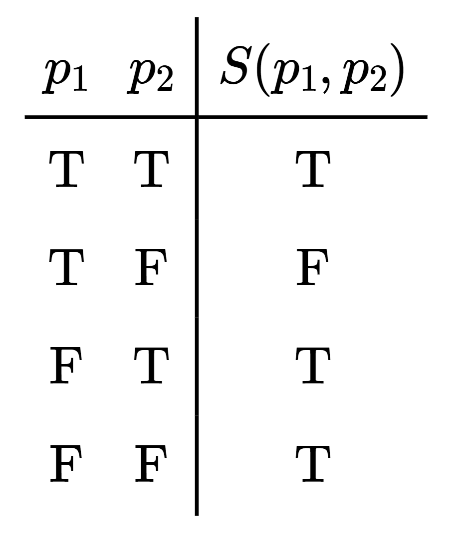
S(p1,p2)=(p1→p2)
is a function S:Λ×Λ→Λ, where
S(T,T)=T,S(T,F)=F,S(F,T)=T,S(F,F)=T.
10.1.3: Graph of a function
the set of all input-output pairs for the function
the graph of function f:A→B, so that
Δ(f)={(a,f(a))|a∈A}⊆A×B
To describe the graph of the function f:N→A defined in Example 10.1.4, we just need to collect the defined input-output pairs into Cartesian product elements:
This graph can most simply be represented by a table:
| x | 1 | 2 | 3 |
| f(x) | d | a | d |
The graph of a function f:R→R is a subset of R×R=R2. We usually represent R2 visually as the xy-plane and the graph Δ(f)⊆R2 as a curve in the plane.
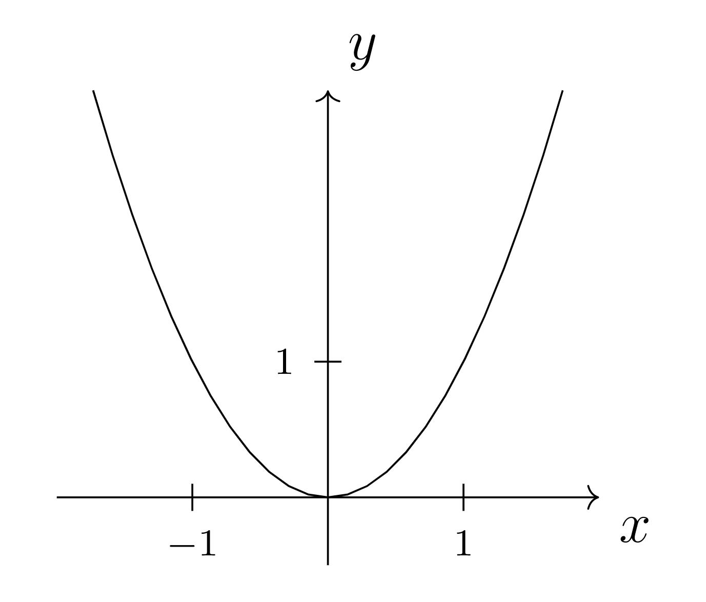
In the graph of f(x)=x2 above, each point on the curve represents an element of R2 which is in the subset Δ(f). For example, (−1,1)∈Δ(f) but (−1,π)∉Δ(f).
The graph of a function f:R2→R is technically a subset of R2×R, but usually we just think of this as R3, or 3-space. Instead of a curve, such a graph defines a surface in R3. For example, the graph of the function f(x,y)=x2+y2 from Example 10.1.5 is a parabolic cone, i.e. a (non-solid) cone-like surface with parabolic sides.
We've already encountered the graph of a logical statement: it is usually represented as a truth table. For example, the graph Δ(S) of the logical statement
where Λ={T,F} as usual, can be represented as below.
Unfortunately, our working definition for function is lacking: what is a “rule”? Rather than chasing some circle of definitions, we can come up with a better definition by noticing that the graph of a function contains all the necessary information about the function.
a subset F⊆A×B such that for every x∈A there is exactly one element (a,b)∈F with a=x
In this formal definition, we are defining a function to be what we previously would have called its graph.
We are now defining a function f:R→R to be the subset of the Cartesian plane R2 consisting of the graph of the function. In this case, you can think of the “exactly one” requirement as equivalent to the vertical line test: an input value may not produce more than one output value. (Though the “one” part of “exactly one” captures our requirement that a function be defined on every domain element.)
10.1.4: Undefined and well-defined
We have to be careful defining functions; sometimes what we think is a function turns out to not be a function.
Again write N={1,2,3} and A={a,b,c,d}, and consider
F={(1,a),(3,d)}⊆N×A.
Does this subset define a function with domain N and codomain A? That is, does there exist a function f:N→A such that F=Δ(f)? The answer is no, because there is no input-output pair in F with domain element 2. If we attempt to consider a function f with graph Δ(f)=F, we have no way to tell what result f(2) should return. In other words, such an f will have been left undefined on element 2, which is supposed to be part of the domain.
The set F does define a function, just not one with domain N. If we consider the smaller set N′={1,3}, then there is a function f:N′→A with F=Δ(f).
Again write N={1,2,3} and A={a,b,c,d}, and consider
F={(1,a),(3,a),(3,d)}⊆N×A.
Does this subset define a function with domain N and codomain A? That is, does there exist a function f:N→A such that F=Δ(f)? The answer is no, because there are more than one input-output pairs with domain element 3. In other words, a function f with graph Δ(f)=F is not well-defined, because we have no way to tell whether f(3) should be a or d.
Recall that
Q={mn|m,n∈Z,n≠0}.
Suppose we attempt to define f:Q→Z by f(mn)=m+n. This seems like a valid way to define a function, until we realize that, for example,
f(12)=1+2=3,f(24)=2+4=6.
This is nonsense, because 12 and 24 represent the same element of Q. Thus, rule f is not well-defined as a function, since to each element of the domain Q it associates more than one element of the codomain Z.
10.1.5: Equality of functions
for f:A→B and g:A→B, write f=g if f(a)=g(a) for all a∈A
The functions f:R→R, f(x)=|x|, and g:R→R, g(x)=√x2, are equal.
10.1.6: Image of a function
the set of all possible outputs of the function
the image of function f:A→B, so that
f(A)={f(a)|a∈A}⊆B
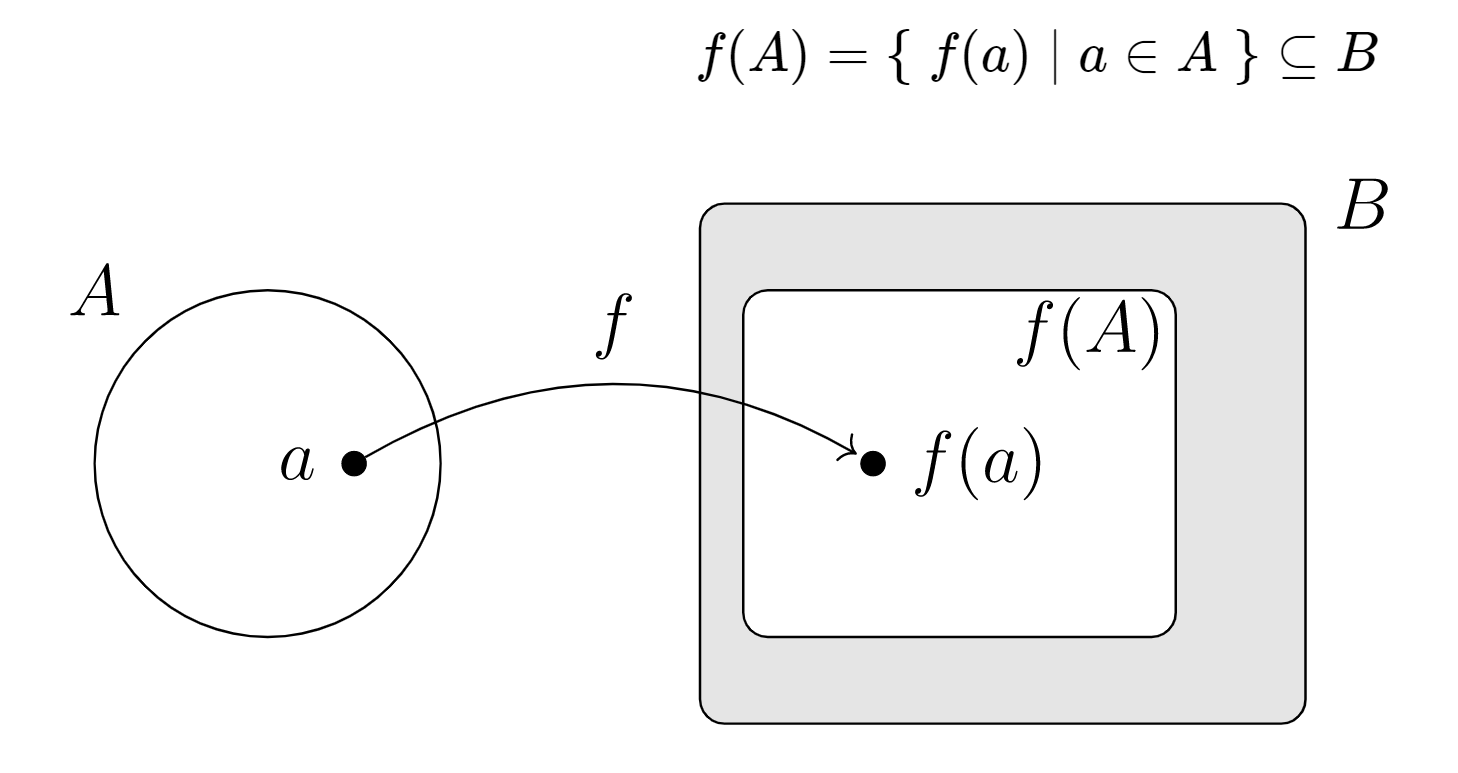
We have stated before that a codomain in a function definition may be “larger” than necessary because we do not always know precisely what output elements a given input-output rule will produce. Our idea of codomain is that it should at least tell us what “type” of outputs will be produced, but not necessarily exactly what outputs will be produced.
With our new concept of function image, we can now repeat this more technically: a function image is always a subset of the codomain, but it might be a proper subset.
How do we know if a codomain element is an image element?
For function f:A→B and codomain element b∈B, we have b∈f(A) if and only if there exists a∈A such that b=f(a).
Consider f:R→R, f(x)=x2. Prove f(R)=R≥0, where R≥0 is the set of nonnegative real numbers.
Solution
Following the Test for Set Equality, we need to show both
f(R)⊆R≥0,f(R)⊇R≥0.
To be more explicit about the second set R≥0, we can write
R≥0={x∈R|x≥0}.
Show f(R)⊆R≥0.
Let y represent an arbitrary element of f(R). As an element of the image of f, y is an output corresponding to some input. That is, there exists some x∈R such that
Therefore, since square numbers are always positive, we have y≥0, and hence y∈R≥0.
Show f(R)⊇R≥0.
Let y represent an arbitrary element of R≥0. To show y∈f(R), we need to find x∈R such that f(x)=y. Let x=√y, which is defined since y∈R≥0 implies y≥0. Then
as desired.
the set of all outputs of a function when only fed inputs from a given subset
the image of the subset A′⊆A under a function f:A→B, so that
f(A′)={f(a)|a∈A′}⊆B
We saw in Worked Example 10.1.16 that for f:R→R, f(x)=x2, we have f(R)=R≥0. Now, the set of integers Z is a subset of the domain R, so we can compute
f(Z)={0,1,4,9,16,…,n2,…}⊆R≥0.