3.2: Implementation of Numerical Packages

3.2.1: First Order ODEs in MATLAB

One can use Matlab to obtain solutions and plots of solutions of differential equations. This can be done either symbolically, using dsolve, or numerically, using numerical solvers like ode45. In this section we will provide examples of using these to solve first order differential equations. We will end with the code for drawing direction fields, which are useful for looking at the general behavior of solutions of first order equations without explicitly finding the solutions.

Symbolic Solutions

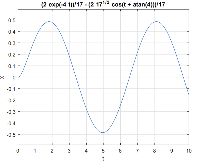
THE FUNCTION dsolve OBTAINS THE SYMBOLIC Solution and ezplot is used to quickly plot the symbolic solution. As an example, we apply dsolve to solve the

\[x^{\prime}=2 \sin t-4 x, \quad x(0)=0 \nonumber \]

At the MATLAB prompt, type the following:

sol = dsolve(’Dx=2*sin(t)-4*x’,’x(0)=0’,’t’);

ezplot(sol,[0 10])

xlabel(’t’),ylabel(’x’), grid

The solution is given as

sol =

(2*exp(-4*t))/17 - (2*17^(1/2)*cos(t + atan(4)))/17

Figure \(\PageIndex{1}\) shows the solution plot.

Figure \(\PageIndex{1}\): The solution of Equation \(\PageIndex{1}\) with \(x(0)=0\) found using MATLAB’s dsolve command.

ODE45 and Other Solvers.

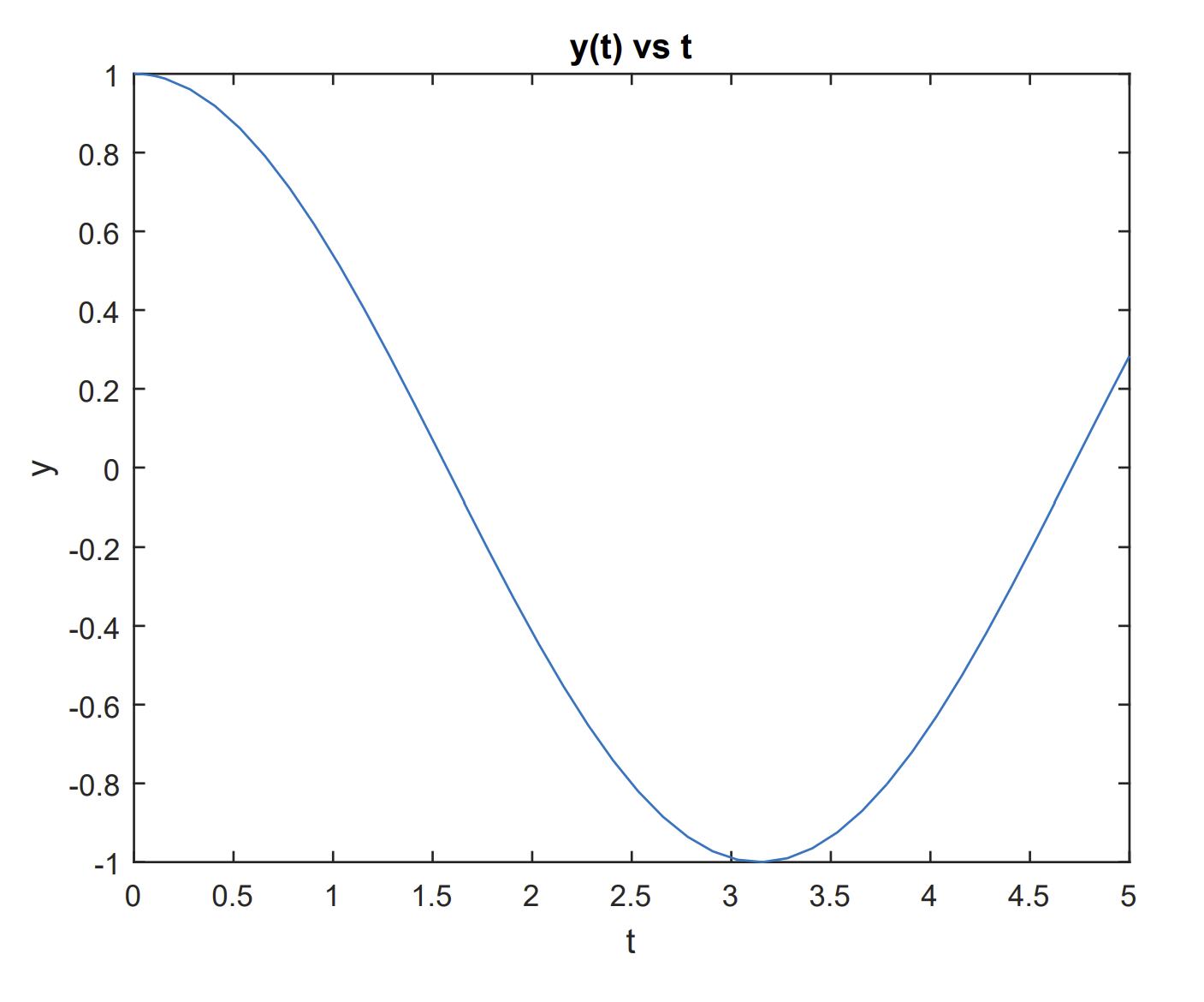
There are several ode solvers in Matlab, implementing Runge-Kutta and other numerical schemes. Examples of its use are in the differential equations textbook. For example, one can implement ode45 to solve the initial value problem

\(\dfrac{d y}{d t}=-\dfrac{y t}{\sqrt{2-y^{2}}}, \quad y(0)=1\)

using the following code:

[t y]=ode45(’func’,[0 5],1);

plot(t,y)

xlabel(’t’),ylabel(’y’)

title(’y(t) vs t’)

One can define the function func in a file func.m such as

function f=func(t,y)

f=-t*y/sqrt(2-y.^2);

Running the above code produces Figure \(\PageIndex{2}\).

Figure \(\PageIndex{2}\): A plot of the solution of \(\dfrac{d y}{d t}=-\dfrac{y t}{\sqrt{2-y^{2}}}, \quad y(0)=1\), found using MATLAB’s ode 45 command.

One can also use ode 45 to solve higher order differential equations. Second order differential equations are discussed in Section 3.2.2. See MATLAB help for other examples and other ODE solvers.

Direction Fields

ONE CAN PRODUCE DIRECTION FIELDS IN MATLAB. For the differential equation

\[\dfrac{d y}{d x}=f(x, y)\nonumber \]

we note that \(f(x, y)\) is the slope of the solution curve passing through the point in the \(x y=\) plane. Thus, the direction field is a collection of tangent vectors at points \((x, y)\) indication the slope, \(f(x, y)\), at that point.

A sample code for drawing direction fields in MATLAB is given by

[x,y]=meshgrid(0:.1:2,0:.1:1.5);

dy=1-y;

dx=ones(size(dy));

quiver(x,y,dx,dy)

axis([0,2,0,1.5])

xlabel(’x’)

ylabel(’y’)

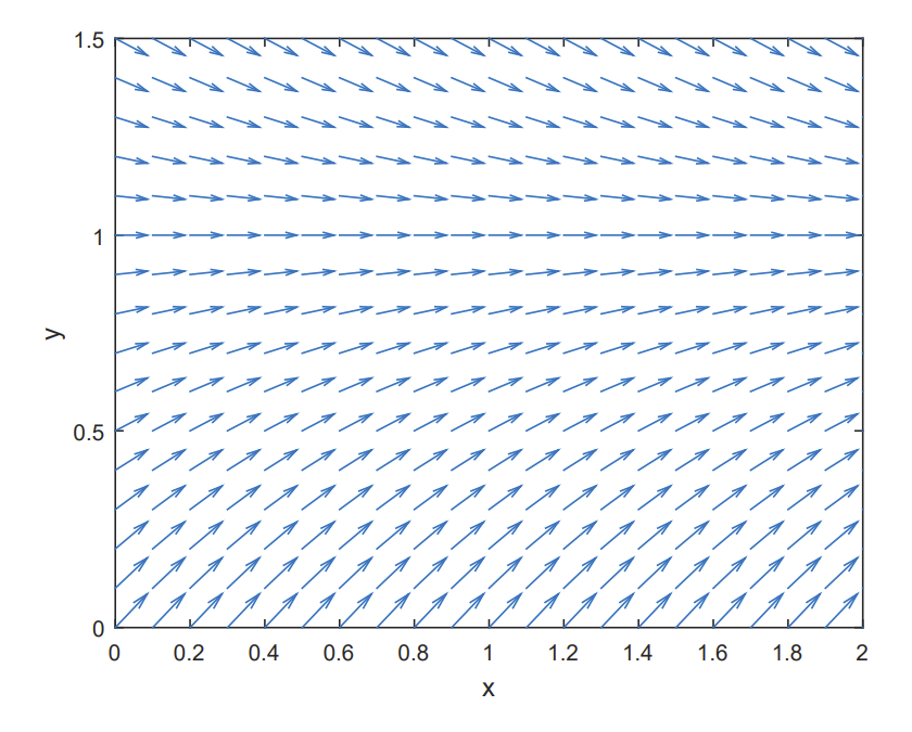
The mesh command sets up the \(x y\)-grid. In this case \(x\) is in \([0,2]\) and \(y\) is in \([0,1.5] .\) In each case the grid spacing is \(0.1 .\)

We let \(d y=1-y\) and \(d x=1\). Thus,

\(\dfrac{d y}{d x}=\dfrac{1-y}{1}=1-y\)

The quiver command produces a vector \((d x, d y)\) at \((x, y)\). The slope of each vector is \(d y / d x\). The other commands label the axes and provides a window with \(x \min =0, x \max =2, y \min =0, y \max =1.5\). The result of using the above code is shown in Figure \(\PageIndex{3}\)) .\)

Figure \(\PageIndex{3}\): A direction field produced using MATLAB’s quiver function for \(y^{\prime}=1-y\).

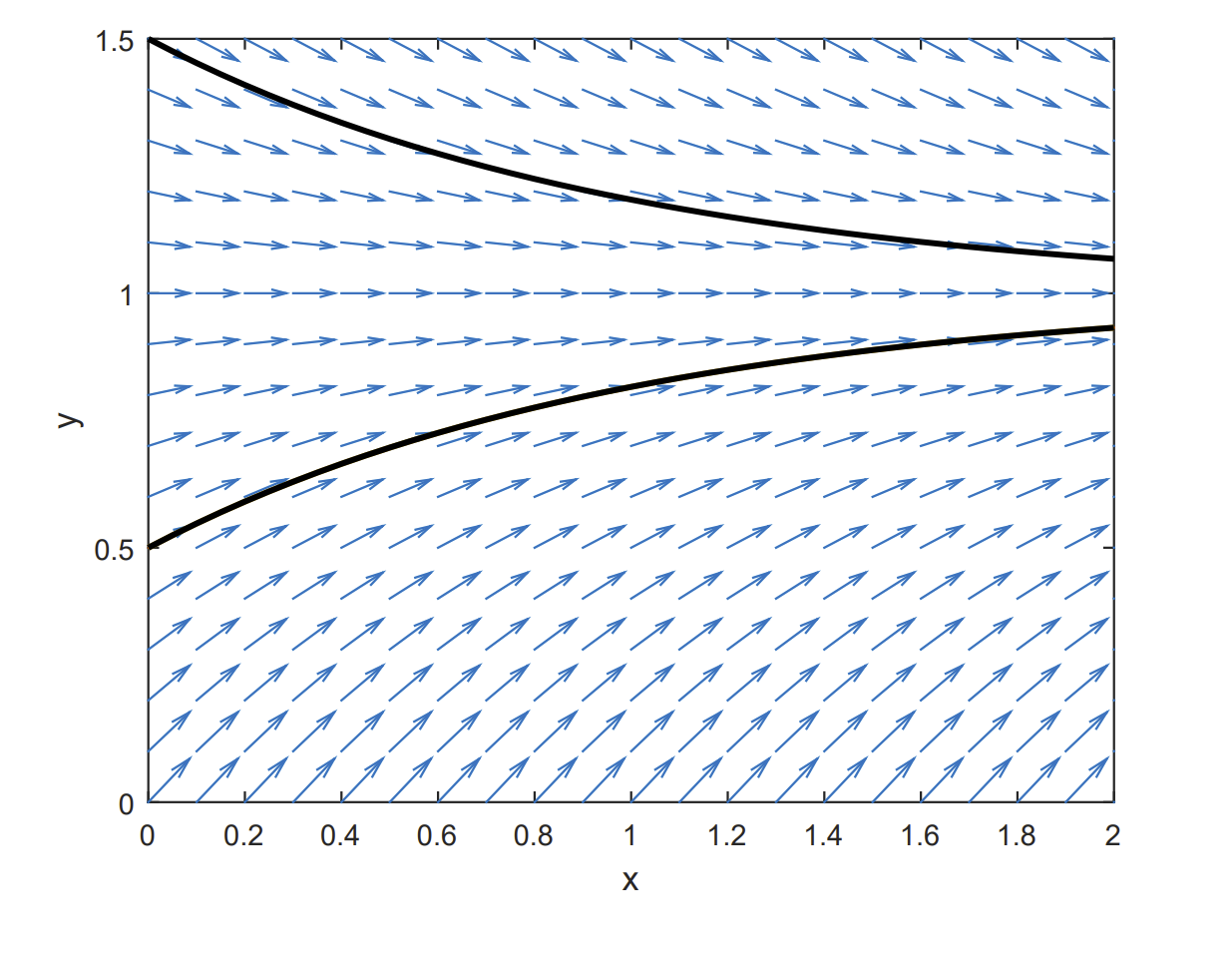
One can add solution, or integral, curves to the direction field for different initial conditions to further aid in seeing the connection between direction fields and integral curves. One needs to add to the direction field code the followig lines:

hold on

[t,y] = ode45(@(t,y) 1-y, [0 2], .5);

plot(t,y,’k’,’LineWidth’,2)

[t,y] = ode45(@(t,y) 1-y, [0 2], 1.5);

plot(t,y,’k’,’LineWidth’,2)

hold off

Here the function \(f(t, y)=1-y\) is entered this time using MATLAB’s anonymous function, @(t,y) 1-y. Before plotting, the hold command is invoked to allow plotting several plots on the same figure. The result is shown the following lines:

Figure \(\PageIndex{4}\): A direction field produced using MATLAB’s quiver function for \(y^{\prime}=1-y\) with solution curves added.

3.2.2: Second Order ODEs in MATLAB

WE CAN ALSO USE ode45 TO SOLVE second and higher order differential equations. The key is to rewrite the single differential equation as a system of first order equations. Consider the simple harmonic oscillator equation, \(\ddot{x}+\omega^{2} x=0 .\) Defining \(y_{1}=x\) and \(y_{2}=\dot{x}\), and noting that

\(\ddot{x}+\omega^{2} x=\dot{y}_{2}+\omega^{2} y_{1}\)

we have

\(\begin{array}{r} \dot{y}_{1}=y_{2} \\ \dot{y}_{2}=-\omega^{2} y_{1} . \end{array}\)

Furthermore, we can view this system in the form \(\dot{\mathbf{y}}=\mathbf{y} .\) In particular, we have

\(\dfrac{d}{d t}\left[\begin{array}{l} y_{1} \\ y_{2} \end{array}\right]=\left[\begin{array}{c} y_{1} \\ -\omega^{2} y_{2} \end{array}\right]\)

Now, we can use ode45. We modify the code slightly from Chapter \(1 .\)

[t y]=ode45(’func’,[0 5],[1 0]);

Here\([0 5]\) gives the time interval and \([1 0]\) gives the initial conditions

\[y_{1}(0)=x(0)=1, \quad y_{2}(0)=\dot{x}(0)=1\nonumber \]

The function func is a set of commands saved to the file func.m for computing the righthand side of the system of differential equations. For the simple harmonic oscillator, we enter the function as

function dy=func(t,y)

omega=1.0;

dy(1,1) = y(2);

dy(2,1) = -omega^2*y(1);

There are a variety of ways to introduce the parameter \(\omega\). Here we simply defined it within the function. Furthermore, the output dy should be a column vector.

After running the solver, we then need to display the solution. The output should be a column vector with the position as the first element and the velocity as the second element. So, in order to plot the solution as a function of time, we can plot the first column of the solution, \(y(:, 1)\), vs \(t\) :

plot(t,y(:,1))

xlabel(’t’),ylabel(’y’)

title(’y(t) vs t’)

Figure \(\PageIndex{5}\): Solution plot for the simple harmonic oscillator.

The resulting solution is shown in Figure \(\PageIndex{5}\).

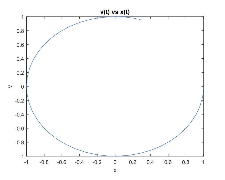
We can also do a phase plot of velocity vs position. In this case, one can plot the second column, \(y(:, 2)\), vs the first column, \(y(:, 1)\) :

plot(y(:,1),y(:,2))

xlabel(’y’),ylabel(’v’)

title(’v(t) vs y(t)’)

The resulting solution is shown in Figure \(\PageIndex{6}\).

Figure \(\PageIndex{6}\): Phase plot for the simple harmonic oscillator.

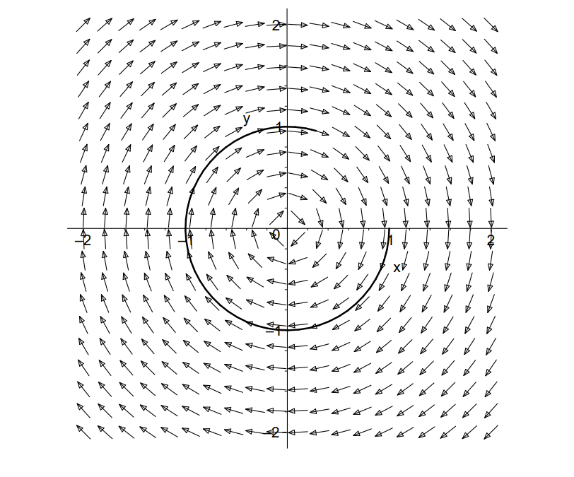
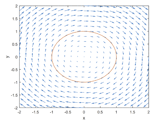
Finally, we can plot a direction field using a quiver plot and add solution curves using ode45. The direction field is given for \(\omega=1\) by \(\mathrm{dx}=\mathrm{y}\) and \(\mathrm{dy}=-\mathrm{X}\).

clear

[x,y]=meshgrid(-2:.2:2,-2:.2:2);

dx=y;

dy=-x;

quiver(x,y,dx,dy)

axis([-2,2,-2,2])

xlabel(’x’)

ylabel(’y’)

hold on

[t y]=ode45(’func’,[0 6.28],[1 0]);

plot(y(:,1),y(:,2))

hold off

The resulting plot is given in Figure \(\PageIndex{7}\).

Figure \(\PageIndex{7}\): Phase plot for the simple harmonic oscillator.

3.2.3: GNU Octave

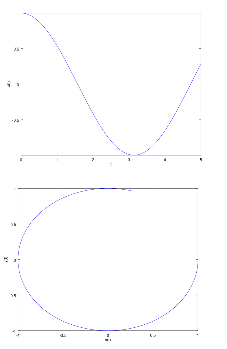
MUCH OF MATLAB’s FUNCTIONALITY CAN BE USED IN GNU OCTAVE. However, a simple solution of a differential equation is not the same. Instead GNU Octave uses the Fortan lsode routine. The main code below gives what is needed to solve the system

\(\dfrac{d}{d t}\left[\begin{array}{l} x \\ y \end{array}\right]=\left[\begin{array}{c} x \\ -c y \end{array}\right]\)

global c

c=1;

y=lsode("oscf",[1,0],(tau=linspace(0,5,100))’);

figure(1);

plot(tau,y(:,1));

xlabel(’t’)

ylabel(’x(t)’)

figure(2);

plot(y(:,1),y(:,2));

xlabel(’x(t)’)

ylabel(’y(t)’)

The function called by the lsode routine, oscf, looks similar to MATLAB code. However, one needs to take care in the syntax and ordering of the input variables. The output from this code is shown in Figure \(\PageIndex{8} .\)

function ydot=oscf(y,tau);

global c

ydot(1)=y(2);

ydot(2)=-c*y(1);

Figure \(\PageIndex{8}\): Numerical solution of the simple harmonic oscillator using GNU Octave’s lsode routine. In these plots are the position and velocity vs times plots and a phase plot.

3.2.4: Python Implementation

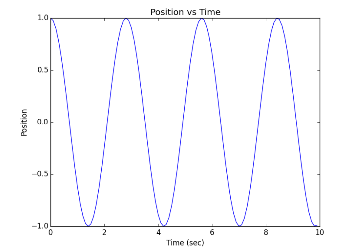
ONE CAN ALSO SOLVE ORDINARY DIFFERENTIAL EQUATIONS using Python. One can use the odeint routine from scipy.inegrate. This uses a variable step routine based on the Fortan lsoda routine. The below code solves a simple harmonic oscillator equation and produces the plot in Figure \(\PageIndex{9}.\)

import numpy as np

import matplotlib. pyplot as plt

from scipy.integrate import odeint

# Solve dv/dt = [y, - cx] for v = [x,y]

def odefn(v,t, c):

x, y = v

dvdt = [y, -c*x ]

return dvdt

v0 = [1.0, 0.0]

t = np.arange(0.0, 10.0, 0.1)

c = 5;

sol = odeint(odefn, v0, t,args=(c,))

plt.plot(t, sol[:,0],’b’)

plt.xlabel(’Time (sec)’)

plt.ylabel(’Position’)

plt.title(’Position vs Time’)

plt.show()

Figure \(\PageIndex{9}\): Numerical solution of the simple harmonic oscillator using Python’s odeint.

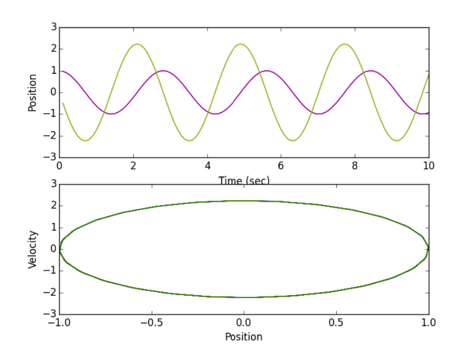
If one wants to use something similar to the Runga-Kutta scheme, then the ode routine can be used with a specification of ode solver. The below code solves a simple harmonic oscillator equation and produces the plot in Figure \(\PageIndex{10}.\)

from scipy import *

from scipy.integrate import ode

from pylab import *

# Solve dv/dt = [y, - cx] for v = [x,y]

def odefn(t,v, c):

x, y = v

dvdt = [y, -c*x ]

return dvdt

v0 = [1.0, 0.0]

t0=0;

tf=10;

dt=0.1;

c = 5;

Y=[];

T=[];

r = ode(odefn).set_integrator(’dopri5’)

r.set_f_params(c).set_initial_value(v0,t0)

while r.successful() and r.t+dt < tf:

r.integrate(r.t+dt)

Y.append(r.y)

T.append(r.t)

Y = array(Y)

subplot(2,1,1)

plot(T,Y)

plt.xlabel(’Time (sec)’)

plt.ylabel(’Position’)

subplot(2,1,2)

plot(Y[:,0],Y[:,1])

xlabel(’Position’)

ylabel(’Velocity’)

show()

3.2.5: Maple Implementation

MAPLE ALSO HAS BUILT-IN ROUTINES FOR SOLVING DIFFERENTIAL EQUATIONS. First, we consider the symbolic solutions of a differential equation. An example of a symbolic solution of a first order differential equation, \(y^{\prime}=1-y\) with \(y(0)-1.5\), is given by

> restart: with(plots):

> EQ:=diff(y(x),x)=1-y(x):

> dsolve({EQ,y(0)=1.5});

Figure \(\PageIndex{10}\): Numerical solution of the simple harmonic oscillator using Python’s ode routine. In these plots are the position and velocity vs times plots and a phase plot.

The resulting solution from Maple is

\[y(x)=1+\dfrac{1}{2} e^{-x} \nonumber \]

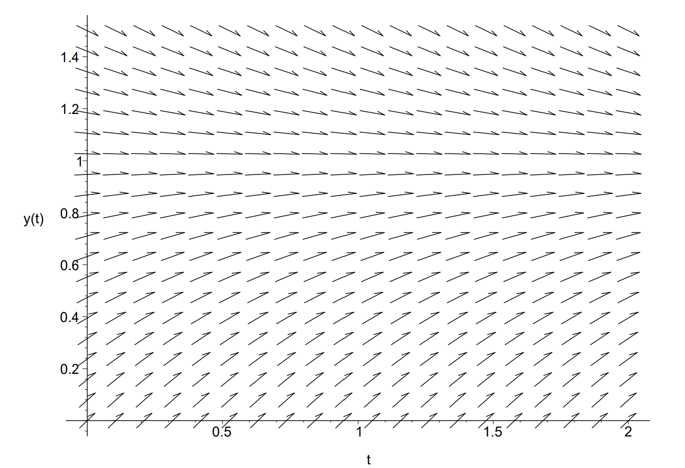
One can also plot direction fields for first order equations. An example is given below with the plot shown in Figure \(\PageIndex{11}\).

Figure \(\PageIndex{11}\): Maple direction field plot for first order differential equation.

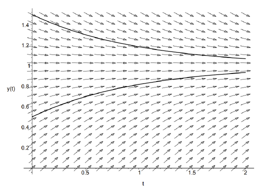
In order to add solution curves, we specify initial conditions using the following lines as seen in Figure \(\PageIndex{12}\).

> ics:=[y(0)=0.5,y(0)=1.5]:

> DEplot(ode,yt),t=0..2,y=0..1.5,ics,arrows=medium,linecolor=black,color=black);

These routines can be used to obtain solutions of a system of differential equations.

Figure \(\PageIndex{12}\): Maple direction field plot for first order differential equation with solution curves added.

> EQ:=diff(x(t),t)=y(t),diff(y(t),t)=-x(t):

> ICs:=x(0)=1,y(0)=0;

> dsolve([EQ, ICs]);

> plot(rhs(%[1]),t=0..5);

A phaseportrait with a direction field, as seen in Figure \(\PageIndex{13}\), is found using the lines

> with(DEtools):

> DEplot( [EQ], [x(t),y(t)], t=0..5, x=-2..2, y=-2..2, , arrows=medium,linecolor=black,color=black,scaling=constrained);

Figure \(\PageIndex{13}\): Maple system plot.