3.1: Euler’s Method

In this section we will look at the simplest method for solving first order equations, Euler’s Method. While it is not the most efficient method, it does provide us with a picture of how one proceeds and can be improved by introducing better techniques, which are typically covered in a numerical analysis text.

Let’s consider the class of first order initial value problems of the form

$$\dfrac{d y}{d x}=f(x, y), \quad y\left(x_{0}\right)=y_{0} \nonumber$$

We are interested in finding the solution $y(x)$ of this equation which passes through the initial point $\left(x_{0}, y_{0}\right)$ in the $x y$-plane for values of $x$ in the interval $[a, b]$, where $a=x_{0}$. We will seek approximations of the solution at $N$ points, labeled $x_{n}$ for $n=1, \ldots, N$. For equally spaced points we have $\Delta x=x_{1}-x_{0}=x_{2}-x_{1}$, etc. We can write these as

$$x_{n}=x_{0}+n \Delta x \nonumber$$

In Figure $\PageIndex{1}$ we show three such points on the $x$-axis.

Figure $\PageIndex{1}$: The basics of Euler’s Method are shown. An interval of the $x$ axis is broken into $N$ subintervals. The approximations to the solutions are found using the slope of the tangent to the solution, given by $f(x, y)$. Knowing previous approximations at $\left(x_{n-1}, y_{n-1}\right)$, one can determine the next approximation, $y_{n}$.

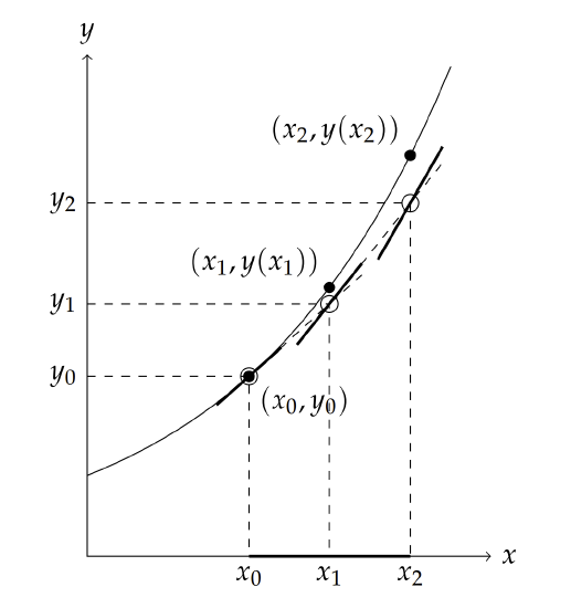
The first step of Euler’s Method is to use the initial condition. We represent this as a point on the solution curve, $\left(x_{0}, y\left(x_{0}\right)\right)=\left(x_{0}, y_{0}\right)$, as shown in Figure $\PageIndex{1}$. The next step is to develop a method for obtaining approximations to the solution for the other $x_{n}^{\prime} s$.

We first note that the differential equation gives the slope of the tangent line at $(x, y(x))$ of the solution curve since the slope is the derivative, $y^{\prime}(x)^{\prime}$ From the differential equation the slope is $f(x, y(x))$. Referring to Figure $\PageIndex{1}$, we see the tangent line drawn at $\left(x_{0}, y_{0}\right)$. We look now at $x=x_{1}$. The vertical line $x=x_{1}$ intersects both the solution curve and the tangent line passing through $\left(x_{0}, y_{0}\right)$. This is shown by a heavy dashed line.

While we do not know the solution at $x=x_{1}$, we can determine the tangent line and find the intersection point that it makes with the vertical. As seen in the figure, this intersection point is in theory close to the point on the solution curve. So, we will designate $y_{1}$ as the approximation of the solution $y\left(x_{1}\right)$. We just need to determine $y_{1}$.

The idea is simple. We approximate the derivative in the differential equation by its difference quotient:

$$\dfrac{d y}{d x} \approx \dfrac{y_{1}-y_{0}}{x_{1}-x_{0}}=\dfrac{y_{1}-y_{0}}{\Delta x} \nonumber$$

Since the slope of the tangent to the curve at $\left(x_{0}, y_{0}\right)$ is $y^{\prime}\left(x_{0}\right)=f\left(x_{0}, y_{0}\right)$, we can write

$$\dfrac{y_{1}-y_{0}}{\Delta x} \approx f\left(x_{0}, y_{0}\right) \nonumber$$

Solving this equation for $y_{1}$, we obtain

$$y_{1}=y_{0}+\Delta x f\left(x_{0}, y_{0}\right) \text {. } \nonumber$$

This gives $y_{1}$ in terms of quantities that we know.

We now proceed to approximate $y\left(x_{2}\right)$. Referring to Figure $\PageIndex{1}$, we see that this can be done by using the slope of the solution curve at $\left(x_{1}, y_{1}\right)$. The corresponding tangent line is shown passing though $\left(x_{1}, y_{1}\right)$ and we can then get the value of $y_{2}$ from the intersection of the tangent line with a vertical line, $x=x_{2}$. Following the previous arguments, we find that

$$y_{2}=y_{1}+\Delta x f\left(x_{1}, y_{1}\right) \text {. } \nonumber$$

Continuing this procedure for all $x_{n}, n=1, \ldots N$, we arrive at the following scheme for determining a numerical solution to the initial value problem:

$$\begin{equation} \begin{aligned} &y_{0}=y\left(x_{0}\right), \\[4pt] &y_{n}=y_{n-1}+\Delta x f\left(x_{n-1}, y_{n-1}\right), \quad n=1, \ldots, N . \end{aligned} \end{equation}\label{3.6}$$

This is referred to as Euler’s Method.

Example $\PageIndex{1}$

Use Euler’s Method to solve the initial value problem $\dfrac{d y}{d x}=x+y, \quad y(0)=1$ and obtain an approximation for $y(1)$.

Solution

First, we will do this by hand. We break up the interval $[0,1]$, since we want the solution at $x=1$ and the initial value is at $x=0$. Let $\Delta x=0.50$. Then, $x_{0}=0, x_{1}=0.5$ and $x_{2}=1.0$. Note that there are $N=\dfrac{b-a}{\Delta x}=2$ subintervals and thus three points.

We next carry out Euler’s Method systematically by setting up a table for the needed values. Such a table is shown in Table 3.1. Note how the table is set up. There is a column for each $x_{n}$ and $y_{n}$. The first row is the initial condition. We also made use of the function $f(x, y)$ in computing the $y_{n}^{\prime}$ s from Equation $\PageIndex{6}$. This sometimes makes the computation easier. As a result, we find that the desired approximation is given as $y_{2}=2.5$.

Table $\PageIndex{1}$: Application of Euler’s Method for $y^{\prime}=x+y, y(0)=1$ and $\Delta x=0.5$.

$n$	$x_{n}$	$y_{n}=y_{n-1}+\Delta x f\left(x_{n-1}, y_{n-1}\right)=0.5 x_{n-1}+1.5 y_{n-1}$
$\mathrm{O}$	$\mathrm{o}$	1
1	$0.5$	$0.5(0)+1.5(1.0)=1.5$
2	$1.0$	$0.5(0.5)+1.5(1.5)=2.5$

Is this a good result? Well, we could make the spatial increments smaller. Let’s repeat the procedure for $\Delta x=0.2$, or $N=5$. The results are in Table $3.2$.

Now we see that the approximation is $y_{1}=2.97664$. So, it looks like the value is near 3 , but we cannot say much more. Decreasing $\Delta x$ more shows that we are beginning to converge to a solution. We see this in Table $\PageIndex{3}$.

Table $\PageIndex{2}$: Application of Euler’s Method for $y^{\prime}=x+y, y(0)=1$ and $\Delta x=0.2$.

$n$	$x_{n}$	$y_{n}=0.2 x_{n-1}+1.2 y_{n-1}$
$\mathrm{o}$	$\mathrm{o}$	1
1	$0.2$	$0.2(0)+1.2(1.0)=1.2$
2	$0.4$	$0.2(0.2)+1.2(1.2)=1.48$
3	$0.6$	$0.2(0.4)+1.2(1.48)=1.856$
4	$0.8$	$0.2(0.6)+1.2(1.856)=2.3472$
5	$1.0$	$0.2(0.8)+1.2(2.3472)=2.97664$

Table $\PageIndex{3}$: Results of Euler’s Method for $y^{\prime}=x+y, y(0)=1$ and varying $\Delta x$

$\Delta x$	$y_{N} \approx y(1)$
$0.5$	$2.5$
$0.2$	$2.97664$
$0.1$	$3.187484920$
$0.01$	$3.409627659$
$0.001$	$3.433847864$
$0.0001$	$3.436291854$

Of course, these values were not done by hand. The last computation would have taken 1000 lines in the table, or at least 40 pages! One could use a computer to do this. A simple code in Maple would look like the following:

Code $\PageIndex{1}$

> restart:

> f:=(x,y)->y+x;

> a:=0: b:=1: N:=100: h:=(b-a)/N;

> x[0]:=0: y[0]:=1:

for i from 1 to N do

y[i]:=y[i-1]+h*f(x[i-1],y[i-1]):

x[i]:=x[0]+h*(i):

od:

evalf(y[N]);

Figure $\PageIndex{2}$: A comparison of the results Euler’s Method to the exact solution for $y^{\prime}=x+y, y(0)=1$ and $N=10$.

In this case we could simply use the exact solution. The exact solution is

$$y(x)=2 e^{x}-x-1 \nonumber$$

(The reader can verify this.) So, the value we are seeking is

$$y(1)=2 e-2=3.4365636 \ldots \nonumber$$

Adding a few extra lines for plotting, we can visually see how well the approximations compare to the exact solution. The Maple code for doing such a plot is given below.

Code $\PageIndex{2}$:

> with(plots):

> Data:=[seq([x[i],y[i]],i=0..N)]:

> P1:=pointplot(Data,symbol=DIAMOND):

> Sol:=t->-t-1+2*exp(t);

> P2:=plot(Sol(t),t=a..b,Sol=0..Sol(b)):

> display({P1,P2});

Figure $\PageIndex{3}$: A comparison of the results Euler’s Method to the exact solution for $y^{\prime}=x+y, y(0)=1$ and $N=100$.

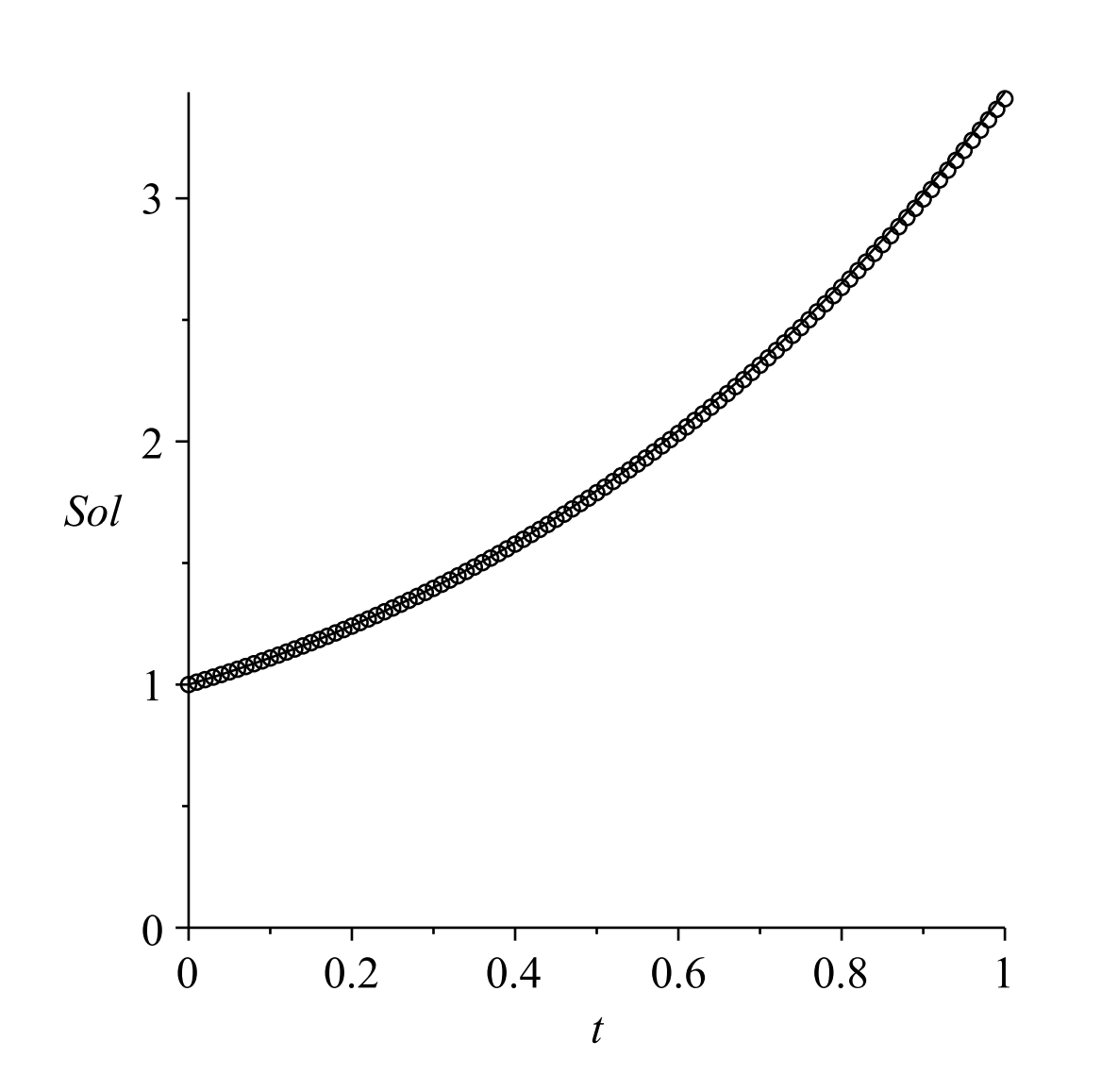
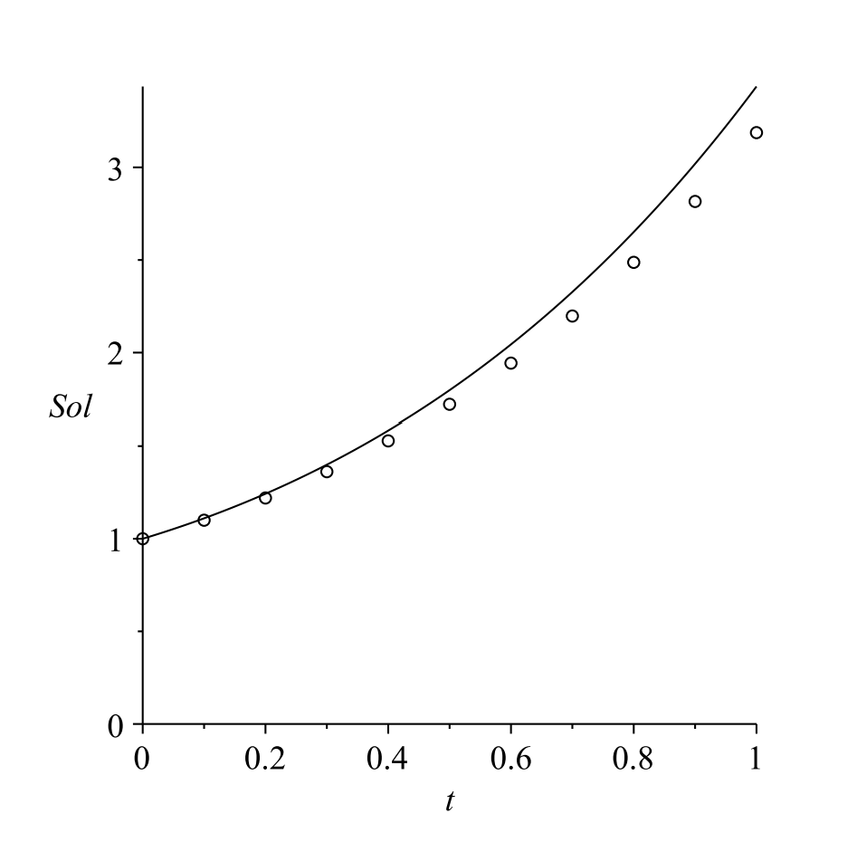
We show in Figures $3.2-3.3$ the results for $N=10$ and $N=100$. In Figure $3.2$ we can see how quickly the numerical solution diverges from the exact solution. In Figure $3.3$ we can see that visually the solutions agree, but we note that from Table $\PageIndex{3}$ that for $\Delta x=0.01$, the solution is still off in the second decimal place with a relative error of about o.8%.

Why would we use a numerical method when we have the exact solution? Exact solutions can serve as test cases for our methods. We can make sure our code works before applying them to problems whose solution is not known.

There are many other methods for solving first order equations. One commonly used method is the fourth order Runge-Kutta method. This method has smaller errors at each step as compared to Euler’s Method. It is well suited for programming and comes built-in in many packages like Maple and MATLAB. Typically, it is set up to handle systems of first order equations.

In fact, it is well known that $n$th order equations can be written as a system of $n$ first order equations. Consider the simple second order equation

$$y^{\prime \prime}=f(x, y) \nonumber$$

This is a larger class of equations than the second order constant coefficient equation. We can turn this into a system of two first order differential equations by letting $u=y$ and $v=y^{\prime}=u^{\prime}$. Then, $v^{\prime}=y^{\prime \prime}=f(x, u)$. So, we have the first order system

$$\begin{aligned} u^{\prime} &=v \\[4pt] v^{\prime} &=f(x, u) \end{aligned} \label{3.7}$$

We will not go further into higher order methods until later in the chapter. We will discuss in depth higher order Taylor methods in Section $3.3$ and Runge-Kutta Methods in Section $3.4$. This will be followed by applications of numerical solutions of differential equations leading to interesting behaviors in Section $3.5$. However, we will first discuss the numerical solution using built-in routines.