3.3: Higher Order Taylor Methods

Euler’s method for solving differential equations is easy to understand but is not efficient in the sense that it is what is called a first order method. The error at each step, the local truncation error, is of order \(\Delta x\), for \(x\) the independent variable. The accumulation of the local truncation errors results in what is called the global error. In order to generalize Euler’s Method, we need to rederive it. Also, since these methods are typically used for initial value problems, we will cast the problem to be solved as

\[\dfrac{d y}{d t}=f(t, y), \quad y(a)=y_{0}, \quad t \in[a, b] \label{3.9} \]

The first step towards obtaining a numerical approximation to the solution of this problem is to divide the \(t\)-interval, \([a, b]\), into \(N\) subintervals,

\(t_{i}=a+i h, \quad i=0,1, \ldots, N, \quad t_{0}=a, \quad t_{N}=b\)

where

\(h=\dfrac{b-a}{N}\)

We then seek the numerical solutions

\(\tilde{y}_{i} \approx y\left(t_{i}\right), \quad i=1,2, \ldots, N\)

with \(\tilde{y}_{0}=y\left(t_{0}\right)=y_{0} .\) Figure \(3.17\) graphically shows how these quantities are related.

Euler’s Method can be derived using the Taylor series expansion of of the solution \(y\left(t_{i}+h\right)\) about \(t=t_{i}\) for \(i=1,2, \ldots, N\). This is given by

\[ \begin{aligned} y\left(t_{i+1}\right) &=y\left(t_{i}+h\right) \\ &=y\left(t_{i}\right)+y^{\prime}\left(t_{i}\right) h+\dfrac{h^{2}}{2} y^{\prime \prime}\left(\xi_{i}\right), \quad \xi_{i} \in\left(t_{i}, t_{i+1}\right) \end{aligned}\label{3.10} \]

Here the term \(\dfrac{h^{2}}{2} y^{\prime \prime}\left(\xi_{i}\right)\) captures all of the higher order terms and represents the error made using a linear approximation to \(y\left(t_{i}+h\right)\). Dropping the remainder term, noting that \(y^{\prime}(t)=f(t, y),\) and defining the resulting numerical approximations by \( \tilde{y}_{i} \approx y\left(t_{i}\right)\), we have

\[ \begin{aligned} \tilde{y}_{i+1}=& \tilde{y}_{i}+h f\left(t_{i}, \tilde{y}_{i}\right), \quad i=0,1, \ldots, N-1, \\ \tilde{y}_{0}=& y(a)=y_{0} . \end{aligned} label{3.11} \nonumber \]

This is Euler’s Method.

Euler’s Method is not used in practice since the error is of order \(h\). However, it is simple enough for understanding the idea of solving differential equations numerically. Also, it is easy to study the numerical error, which we will show next.

The error that results for a single step of the method is called the local truncation error, which is defined by

\(\tau_{i+1}(h)=\dfrac{y\left(t_{i+1}\right)-\tilde{y}_{i}}{h}-f\left(t_{i}, y_{i}\right)\)

A simple computation gives

\(\tau_{i+1}(h)=\dfrac{h}{2} y^{\prime \prime}\left(\xi_{i}\right), \quad \xi_{i} \in\left(t_{i}, t_{i+1}\right)\)

Since the local truncation error is of order \(h\), this scheme is said to be of order one. More generally, for a numerical scheme of the form

\[ \begin{aligned} \tilde{y}_{i+1} &=\tilde{y}_{i}+h F\left(t_{i}, \tilde{y}_{i}\right), \quad i=0,1, \ldots, N-1 \\ \tilde{y}_{0} &=y(a)=y_{0} \end{aligned} \label{3.12} \]

(The local truncation error.) the local truncation error is defined by

\(\tau_{i+1}(h)=\dfrac{y\left(t_{i+1}\right)-\tilde{y}_{i}}{h}-F\left(t_{i}, y_{i}\right)\)

The accumulation of these errors leads to the global error. In fact, one can show that if \(f\) is continuous, satisfies the Lipschitz condition,

\(\left|f\left(t, y_{2}\right)-f\left(t, y_{1}\right)\right| \leq L\left|y_{2}-y_{1}\right|\)

for a particular domain \(D \subset R^{2}\), and

\(\left|y^{\prime \prime}(t)\right| \leq M, \quad t \in[a, b]\)

then

\(\left|y\left(t_{i}\right)-\tilde{y}\right| \leq \dfrac{h M}{2 L}\left(e^{L\left(t_{i}-a\right)}-1\right), \quad i=0,1, \ldots, N\)

Furthermore, if one introduces round-off errors, bounded by \(\delta\), in both the initial condition and at each step, the global error is modified as

\(\left|y\left(t_{i}\right)-\tilde{y}\right| \leq \dfrac{1}{L}\left(\dfrac{h M}{2}+\dfrac{\delta}{h}\right)\left(e^{L\left(t_{i}-a\right)}-1\right)+\left|\delta_{0}\right| e^{L\left(t_{i}-a\right)}, \quad i=0,1, \ldots, N\)

Then for small enough steps \(h\), there is a point when the round-off error will dominate the error. [See Burden and Faires, Numerical Analysis for the details.]

Can we improve upon Euler’s Method? The natural next step towards finding a better scheme would be to keep more terms in the Taylor series expansion. This leads to Taylor series methods of order \(n\).

Taylor series methods of order \(n\) take the form

\[ \begin{aligned} \tilde{y}_{i+1} &=\tilde{y}_{i}+h T^{(n)}\left(t_{i}, \tilde{y}_{i}\right), \quad i=0,1, \ldots, N-1 \\ \tilde{y}_{0} &=y_{0} \end{aligned} \label{3.13} \]

where we have defined

\(T^{(n)}(t, y)=y^{\prime}(t)+\dfrac{h}{2} y^{\prime \prime}(t)+\cdots+\dfrac{h^{(n-1)}}{n !} y^{(n)}(t)\)

However, since \(y^{\prime}(t)=f(t, y)\), we can write

\(T^{(n)}(t, y)=f(t, y)+\dfrac{h}{2} f^{\prime}(t, y)+\cdots+\dfrac{h^{(n-1)}}{n !} f^{(n-1)}(t, y)\)

We note that for \(n=1\), we retrieve Euler’s Method as a special case. We demonstrate a third order Taylor’s Method in the next example.

Example \(\PageIndex{1}\)

Apply the third order Taylor’s Method to

\(\dfrac{d y}{d t}=t+y, \quad y(0)=1\)

Solution

and obtain an approximation for \(y(1)\) for \(h=0.1\).

The third order Taylor’s Method takes the form

\[ \begin{aligned} \tilde{y}_{i+1} &=\tilde{y}_{i}+h T^{(3)}\left(t_{i}, \tilde{y}_{i}\right), \quad i=0,1, \ldots, N-1 \\ \tilde{y}_{0} &=y_{0} \end{aligned} \label{3.14} \]

where

\[T^{(3)}(t, y)=f(t, y)+\dfrac{h}{2} f^{\prime}(t, y)+\dfrac{h^{2}}{3 !} f^{\prime \prime}(t, y)\nonumber \]

and \(f(t, y)=t+y(t)\).

In order to set up the scheme, we need the first and second derivative of \(f(t, y)\):

\[ \begin{aligned} f^{\prime}(t, y) &=\dfrac{d}{d t}(t+y) \\ &=1+y^{\prime} \\ &=1+t+y\end{aligned}\label{3.15} \]

\[ \begin{aligned} f^{\prime \prime}(t, y) &=\dfrac{d}{d t}(1+t+y) \\ &=1+y^{\prime} \\ &=1+t+y \end{aligned} \label{3.16} \]

Inserting these expressions into the scheme, we have

\[ \begin{aligned} \tilde{y}_{i+1} &=\tilde{y}_{i}+h\left[\left(t_{i}+y_{i}\right)+\dfrac{h}{2}\left(1+t_{i}+y_{i}\right)+\dfrac{h^{2}}{3 !}\left(1+t_{i}+y_{i}\right)\right] \\ &=\tilde{y}_{i}+h\left(t_{i}+y_{i}\right)+h^{2}\left(\dfrac{1}{2}+\dfrac{h}{6}\right)\left(1+t_{i}+y_{i}\right) \\ \tilde{y}_{0} &=y_{0} \end{aligned} \label{3.17} \]

for \(i=0,1, \ldots, N-1\).

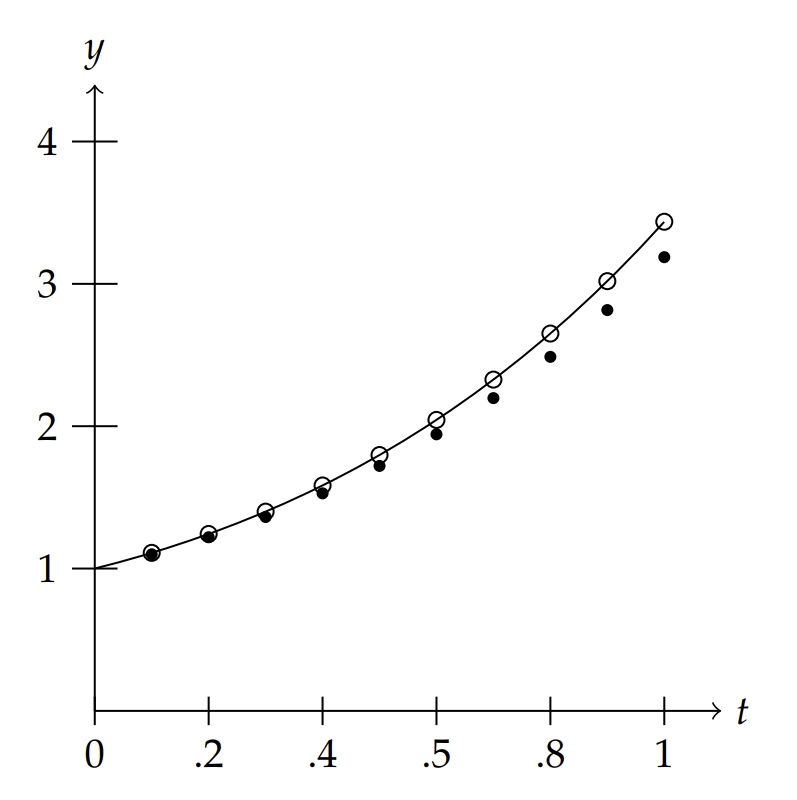
In Figure \(3.1.1\) we show the results comparing Euler’s Method, the 3 rd Order Taylor’s Method, and the exact solution for \(N=10\). In Table \(\PageIndex{1}\) we provide are the numerical values. The relative error in Euler’s method is about \(7 \%\) and that of the 3 rd Order Taylor’s Method is about o.006%. Thus, the 3 rd Order Taylor’s Method is significantly better than Euler’s Method.

In the last section we provided some Maple code for performing Euler’s method. A similar code in MATLAB looks like the following:

a=0;

b=1;

N=10;

h=(b-a)/N;

Table \(\PageIndex{1}\): Numerical values for Euler’s Method, 3rd Order Taylor’s Method, and exact solution for solving Example \(\PageIndex{1}\) with \(N=10\).

Euler	Taylor	Exact
\(1.0000\)	\(1.0000\)	\(1.0000\)
\(1.1000\)	\(1.1103\)	\(1.1103\)
\(1.2200\)	\(1.2428\)	\(1.2428\)
\(1.3620\)	\(1.3997\)	\(1.3997\)
\(1.5282\)	\(1.5836\)	\(1.5836\)
\(1.7210\)	\(1.7974\)	\(1.7974\)
\(1.9431\)	\(2.0442\)	\(2.0442\)
\(2.1974\)	\(2.3274\)	\(2.3275\)
\(2.4872\)	\(2.6509\)	\(2.6511\)
\(2.8159\)	\(3.0190\)	\(3.0192\)
\(3.1875\)	\(3.4364\)	\(3.4366\)

Figure \(\PageIndex{1}\): Numerical results for Euler’s Method (filled circle) and 3 rd Order Taylor’s Method (open circle) for solving Example \(\PageIndex{1}\) as compared to exact solution (solid line).

% Slope function

f = inline(’t+y’,’t’,’y’);

sol = inline(’2*exp(t)-t-1’,’t’);

% Initial Condition

t(1)=0;

y(1)=1;

% Euler’s Method

for i=2:N+1

y(i)=y(i-1)+h*f(t(i-1),y(i-1));

t(i)=t(i-1)+h;

end

A simple modification can be made for the 3 rd Order Taylor’s Method by replacing the Euler’s method part of the preceding code by

% Taylor’s Method, Order 3

y(1)=1;

h3 = h^2*(1/2+h/6);

for i=2:N+1

y(i)=y(i-1)+h*f(t(i-1),y(i-1))+h3*(1+t(i-1)+y(i-1));

t(i)=t(i-1)+h;

end

While the accuracy in the last example seemed sufficient, we have to remember that we only stopped at one unit of time. How can we be confident that the scheme would work as well if we carried out the computation for much longer times. For example, if the time unit were only a second, then one would need 86,400 times longer to predict a day forward. Of course, the scale matters. But, often we need to carry out numerical schemes for long times and we hope that the scheme not only converges to a solution, but that it coverges to the solution to the given problem. Also, the previous example was relatively easy to program because we could provide a relatively simple form for \(T^{(3)}(t, y)\) with a quick computation of the derivatives of \(f(t, y)\). This is not always the case and higher order Taylor methods in this form are not typically used. Instead, one can approximate \(T^{(n)}(t, y)\) by evaluating the known function \(f(t, y)\) at selected values of \(t\) and \(y\), leading to Runge-Kutta methods.