3.5.2: Extreme Sky Diving

ON OCTOBER 14, 2012 FELIX BAUMGARTNER JUMPED from a helium balloon at an altitude of \(39045 \mathrm{~m}(24.26 \mathrm{mi}\) or \(128100 \mathrm{ft})\). According preliminary data from the Red Bull Stratos Mission \({ }^{1}\), as of November 6,2012 Baumgartner experienced free fall until he opened his parachute at \(1585 \mathrm{~m}\) after 4 minutes and 20 seconds. Within the first minute he had broken the record set by Joe Kittinger on August 16,1960 . Kittinger jumped from 102,800 feet \((31 \mathrm{~km})\) and fell freely for 4 minutes and 36 seconds to an altitude of \(18,000 \mathrm{ft}\) conservation.\((5,500 \mathrm{~m})\). Both set records for their times. Kittinger reached \(614 \mathrm{mph}\) (Mach o.9) and Baumgartner reached \(833.9 \mathrm{mph}\) (Mach 1.24). Another record that was broken was that over 8 million watched the event on YouTube, breaking current live stream viewing events.

1

The original estimated data was found at the Red Bull Stratos site, http://www.redbullstratos.com/. Some of the data has since been updated. The reader can redo the solution using the updated data.

This much attention also peaked interest in the physics of free fall. Free fall at constant \(g\) through a height of \(h\) should take a time of

\(t=\sqrt{\dfrac{2 h}{g}}=\sqrt{\dfrac{2(36,529)}{9.8}}=86 \mathrm{~s}\)

Of course, \(g\) is not constant. In fact, at an altitude of \(39 \mathrm{~km}\), we have

\(g=\dfrac{G M}{R+h}=\dfrac{6.67 \times 10^{-11} \mathrm{Nm}^{2} \mathrm{~kg}^{2}\left(5.97 \times 10^{24} \mathrm{~kg}\right)}{6375+39 \mathrm{~km}}=9.68 \mathrm{~m} / \mathrm{s}^{2}\)

So, \(g\) is roughly constant.

Next, we need to consider the drag force as one free falls through the atmosphere, \(F_{D}=\dfrac{1}{2} C A \rho_{a} v^{2} .\) One needs some values for the parameters in this problem. Let’s take \(m=90 \mathrm{~kg}, A=1.0 \mathrm{~m}^{2}\), and \(\rho=1.29 \mathrm{~kg} / \mathrm{m}^{3}\), \(C=0.42\). Then, a simple model would give

\(m \dot{v}=-m g+\dfrac{1}{2} C A \rho v^{2}\)

or

\(\dot{v}=-g+.0030 v^{2}\)

This gives a terminal velocity of \(57.2 \mathrm{~m} / \mathrm{s}\), or \(128 \mathrm{mph}\). However, we again have assumed that the drag coefficient and air density are constant. Since the Reynolds number is high, we expect \(C\) is roughly constant. However, the density of the atmosphere is a function of altitude and we need to take this into account.

The Reynolds number is used several times in this chapter. It is defined as

\(R e=\dfrac{2 r v}{v},\)

where \(v\) is the kinematic viscosity. The kinematic viscosity of air at \(60^{\circ} \mathrm{F}\) is about \(1.47 \times 10^{-5} \mathrm{~m}^{2} / \mathrm{s}\).

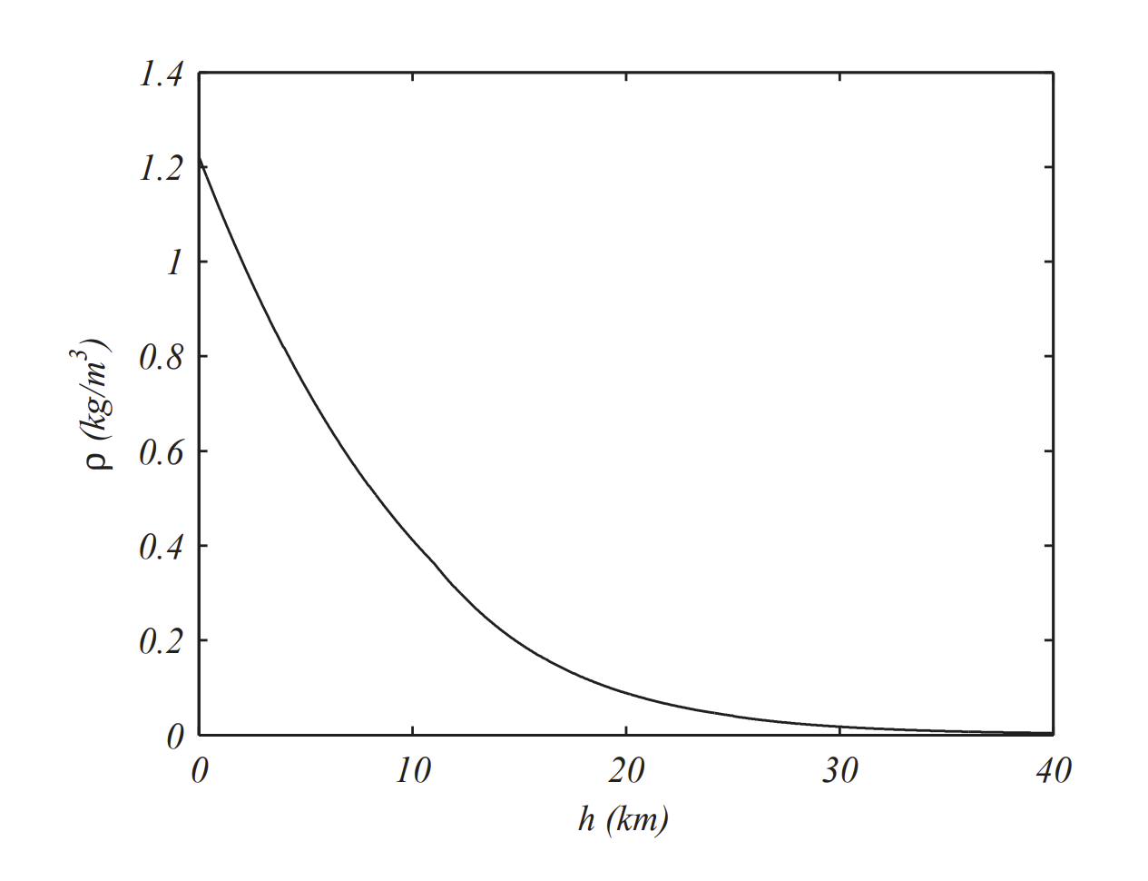
A simple model for \(\rho=\rho(h)\) can be found at the NASA site. \(^{2}\) Using their data, we have

\[\rho(h)=\left\{\begin{array}{cl} \dfrac{101290\left(1.000-0.2253 \times 10^{-4} h\right)^{5.256}}{83007-1.8696 h}, & h<11000 \\ \dfrac{.3629 e^{1.73-0.157 \times 10^{-3} h},}{2488} & h, \\ \dfrac{1388(40876+.8614 h)^{-4}}{\left(.6551+0.1380 \times 10^{-4} h\right)^{11.388}}, & h>25000 \end{array}\right. \end{equation}\label{3.30} \]

In Figure \(\PageIndex{1}\) the atmospheric density is shown as a function of altitude.

2

https://www.grc.nasa.gov/WWW/k-12/rocket/atmos.html

In order to use the methods for solving first order equations, we write the system of equations in the form

\[ \begin{aligned} &\dfrac{d h}{d t}=v \\ &\dfrac{d v}{d t}=-\dfrac{G M}{(R+h)^{2}}+\dfrac{1}{5} \rho(h) C A v^{2} \end{aligned}\label{3.31} \]

This is now in the form of a system of first order differential equations.

Then, we define a function to be called and store in as gravf.m as shown below.

Figure \(\PageIndex{1}\): Atmospheric density as a function of altitude.

function dy=gravf(t,y);

G=6.67E-11;

M=5.97E24;

R=6375000;

m=90;

C=.42;

A=1;

dy(1,1)=y(2);

dy(2,1)=-G*M/(R+y(1)).^2+.5*density2(y(1))*C*A*y(2).^2/m;

Now we are ready to call the function in our favorite routine.

h0=1000;

tmax=20;

tmin=0;

[t,y]=ode45(’dgravf’,[tmin tmax],[h0;0]);% Const rho

plot(t,y(:,1),’k--’)

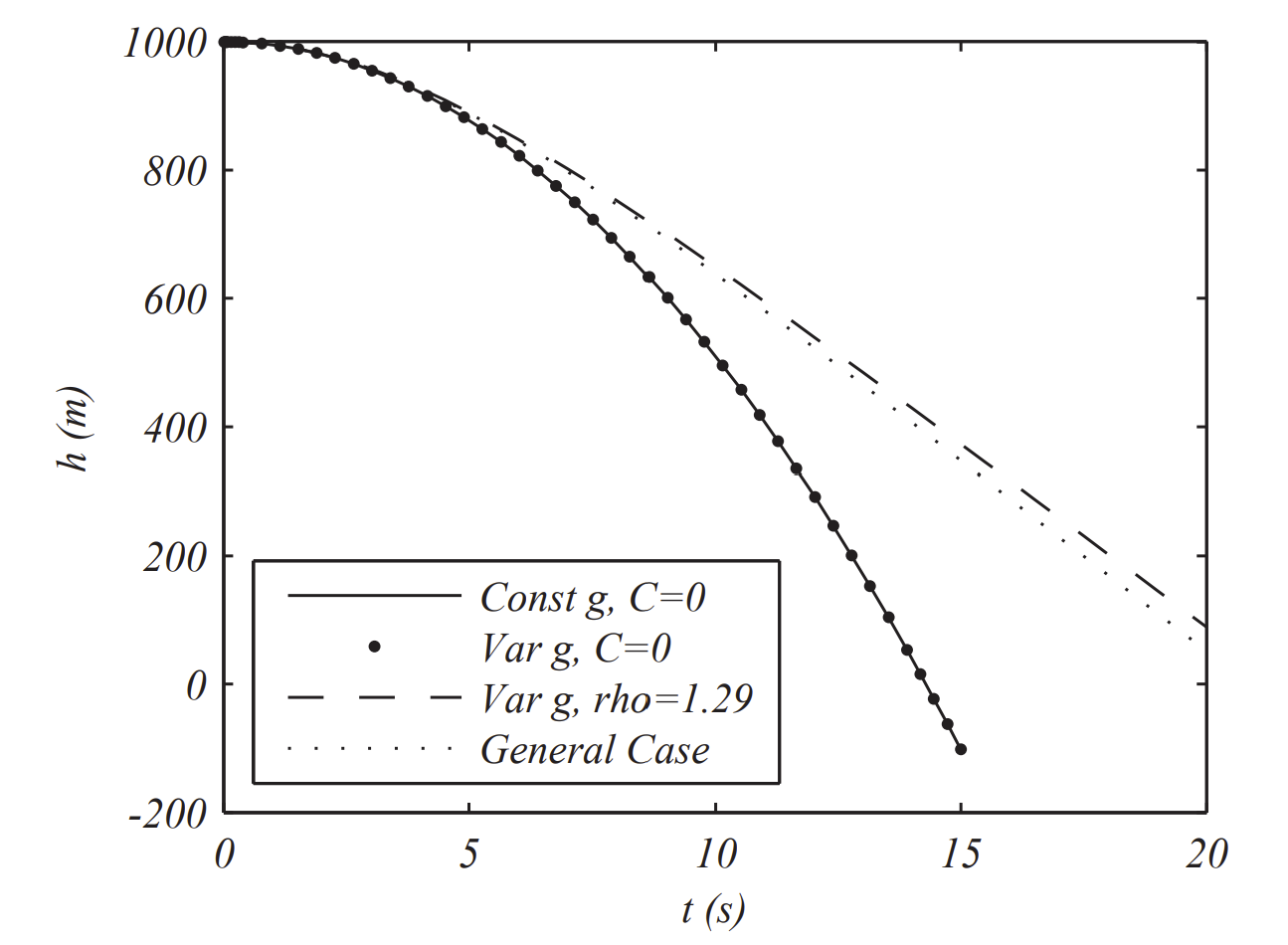
Here we are simulating free fall from an altitude of one kilometer. In Figure \(\PageIndex{2}\) we compare different models of free fall with \(g\) taken as constant or derived from Newton’s Law of Gravitation. We also consider constant density or the density dependence on the altitude as given earlier. We chose to keep the drag coefficient constant at \(C=0.42\).

We can see from these plots that the slight variation in the acceleration due to gravity does not have as much an effect as the variation of density with distance.

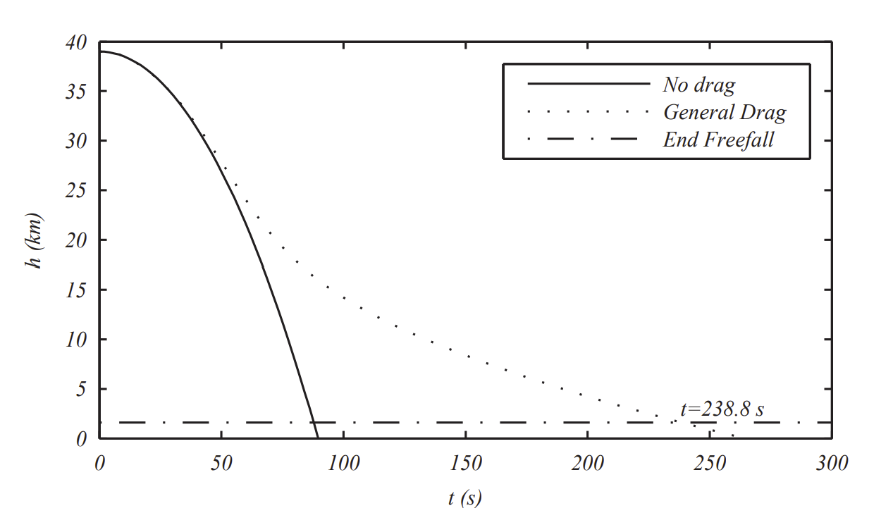
Now we can push the model to Baumgartner’s jump from \(39 \mathrm{~km}\). In Figure \(\PageIndex{3}\) we compare the general model with that with no air resistance, though both taking into account the variation in \(g .\) As a body falls through the atmosphere we see the changing effects of the denser atmosphere on the free fall. For the parameters chosen, we find that it takes \(238.8 \mathrm{~s}\), or a little less than four minutes to reach the point where Baumgartner opened his parachute. While not exactly the same as the real fall, it is amazingly close.

Figure \(\PageIndex{2}\): Comparison of different models of free fall from one kilometer above the Earth.

Figure \(\PageIndex{3}\): Free fall from \(39 \mathrm{~km}\) at constant \(g\) as compared to nonconstant \(g\) and nonconstant atmospheric density with drag coefficient \(C=.42\).