3.5.3: The Flight of Sports Balls

ANOTHER INTERESTING PROBLEM IS THE PROJECTILE MOTION OF A SPORTS ball. In an introductory physics course, one typically ignores air resistance and the path of the ball is a nice parabolic curve. However, adding air resistance complicates the problem significantly and cannot be solved analytically. Examples in sports are flying soccer balls, golf balls, ping pong balls, baseballs, and other spherical balls.

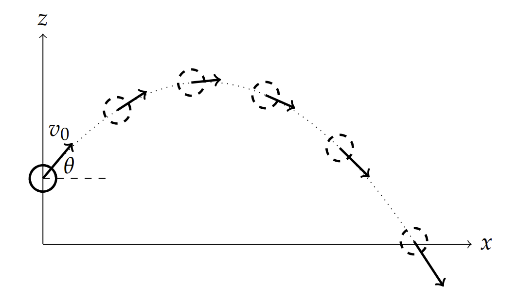
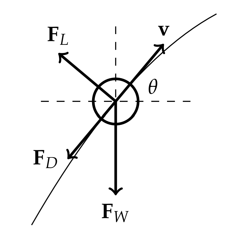
We will consider a ball moving in the \(x z\)-plane spinning about an axis perpendicular to the plane of motion. Such an analysis was reported in Goff and Carré, AJP 77 (11) 1020. The typical trajectory of the ball is shown in Figure \(3.26\). The forces acting on the ball are the drag force, \(\mathbf{F}_{D}\), the lift force, \(\mathbf{F}_{L}\), and the gravitational force, \(\mathbf{F}_{W} .\) These are indicated in Figure \(3.27\). The equation of motion takes the form

\(m \mathbf{a}=\mathbf{F}_{W}+\mathbf{F}_{D}+\mathbf{F}_{L}\)

Writing out the components, we have

\[m a_{x}=-F_{D} \cos \theta-F_{L} \sin \theta \nonumber \]

\[m a_{z}=-m g-F_{D} \sin \theta+F_{L} \cos \theta \nonumber \]

Figure \(\PageIndex{1}\): Sketch of the path for projectile motion problems.

Figure \(\PageIndex{2}\): Forces acting on ball.

As we had seen before, the magnitude of the damping (drag) force is given by

\[F_{D}=\dfrac{1}{2} C_{D} \rho A v^{2}\nonumber \]

For the case of soccer ball dynamics, Goff and Carré noted that the Reynolds number, \(R e=\dfrac{2 r v}{v}\), is between 70000 and 490000 by using a kinematic viscosity of \(v=1.54 \times 10^{-5} \mathrm{~m}^{2} / \mathrm{s}\) and typical speeds of \(v=4.5-31 \mathrm{~m} / \mathrm{s}\). Their analysis gives \(C_{D} \approx 0.2\). The parameters used for the ball were \(m=0.424\) \(\mathrm{kg}\) and cross sectional area \(A=0.035 \mathrm{~m}^{2}\) and the density of air was taken as \(1.2 \mathrm{~kg} / \mathrm{m}^{3}\)

The lift force takes a similar form,

\(F_{L}=\dfrac{1}{2} C_{L} \rho A v^{2} .\)

The sign of \(C_{L}\) indicates if the ball has top spin \(\left(C_{L}<0\right)\) or bottom spin \(\left.{ }^{*} C_{L}>0\right)\). The lift force is just one component of a more general Magnus force, which is the force on a spinning object in a fluid and is perpendicular to the motion. In this example we assume that the spin axis is perpendicular to the plane of motion. Allowing for spinning balls to veer from this plane would mean that we would also need a component of the Magnus force perpendicular to the plane of motion. This would lead to an additional sideways component (in the \(\mathbf{k}\) direction) leading to a third acceleration equation. We will leave that case for the reader.

The lift coefficient can be related to the spin as

\[C_{L}=\dfrac{1}{2+\dfrac{v}{v_{s p i n}}} \nonumber \]

where \(v_{s p i n}=r \omega\) is the peripheral speed of the ball. Here \(R\) is the ball radius and \(\omega\) is the angular speed in rad /s. If \(v=20 \mathrm{~m} / \mathrm{s}, \omega=200 \mathrm{rad} / \mathrm{s}\), and \(r=20 \mathrm{~mm}\), then \(C_{L}=0.45\).

So far, the problem has been reduced to

\[\dfrac{d v_{x}}{d t} =-\dfrac{\rho A}{2 m}\left(C_{D} \cos \theta+C_{L} \sin \theta\right) v^{2} \nonumber \]

\[\dfrac{d v_{z}}{d t} =-g-\dfrac{\rho A}{2 m}\left(C_{D} \sin \theta-C_{L} \cos \theta\right) v^{2} \nonumber \]

for \(v_{x}\) and \(v_{z}\) the components of the velocity. Also, \(v^{2}=v_{x}^{2}+v_{z}^{2}\). Furthermore, from Figure \(\PageIndex{2}\), we can write

\(\cos \theta=\dfrac{v_{x}}{v}, \quad \sin \theta=\dfrac{v_{z}}{v} .\)

So, the equations can be written entirely as a system of differential equations for the velocity components,

\[\dfrac{d v_{x}}{d t} =-\alpha\left(C_{D} v_{x}+C_{L} v_{z}\right)\left(v_{x}^{2}+v_{z}^{2}\right)^{1 / 2} \nonumber \]

\[\dfrac{d v_{z}}{d t} &=-g-\alpha\left(C_{D} v_{z}-C_{L} v_{x}\right)\left(v_{x}^{2}+v_{z}^{2}\right)^{1 / 2} \nonumber \]

where \(\alpha=\rho A / 2 m=0.0530 \mathrm{~m}^{-1}\).

Such systems of equations can be solved numerically by thinking of this as a vector differential equation,

\(\dfrac{d \mathbf{v}}{d t}=\mathbf{F}(t, \mathbf{v})\)

and applying one of the numerical methods for solving first order equations.

Since we are interested in the trajectory, \(z=z(x)\), we would like to determine the parametric form of the path, \((x(t), z(t))\). So, instead of solving two first order equations for the velocity components, we can rewrite the two second order differential equations for \(x(t)\) and \(z(t)\) as four first order differential equations of the form

\(\dfrac{d \mathbf{y}}{d t}=\mathbf{F}(t, \mathbf{y})\)

We first define

\(\mathbf{y}=\left[\begin{array}{l} y_{1}(t) \\ y_{2}(t) \\ y_{3}(t) \\ y_{4}(t) \end{array}\right]=\left[\begin{array}{c} x(t) \\ z(t) \\ v_{x}(t) \\ v_{z}(t) \end{array}\right]\)

Then, the systems of first order differential equations becomes

\[ \begin{aligned} \dfrac{d y_{1}}{d t} &=y_{3} \\ \dfrac{d y_{2}}{d t} &=y_{4} \\ \dfrac{d y_{3}}{d t} &=-\alpha\left(C_{D} v_{x}+C_{L} v_{z}\right)\left(v_{x}^{2}+v_{z}^{2}\right)^{1 / 2} \\ \dfrac{d y_{4}}{d t} &=-g-\alpha\left(C_{D} v_{z}-C_{L} v_{x}\right)\left(v_{x}^{2}+v_{z}^{2}\right)^{1 / 2} \end{aligned} \label{3.38} \]

The system can be placed into a function file which can be called by an ODE solver, such as the MATLAB m-file below.

function dy = ballf(t,y)

global g CD

CL alpha dy = zeros(4,1); % a column vector

v = sqrt(y(3).^2+y(4).^2); % speed v

dy(1) = y(3);

dy(2) = y(4);

dy(3) = -alpha*v.*(CD*y(3)+CL*y(4));

dy(4) = alpha*v.*(-CD*y(4)+CL*y(3))-g;

Then, the solver can be called using

[T,Y] = ode45(’ballf’,[0 2.5],[x0,z0,v0x,v0z]);

Figure \(\PageIndex{3}\): Example of soccer ball under the influence of drag.

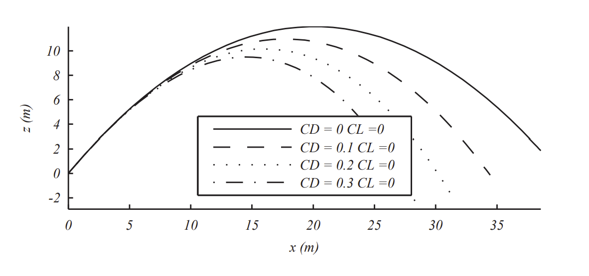
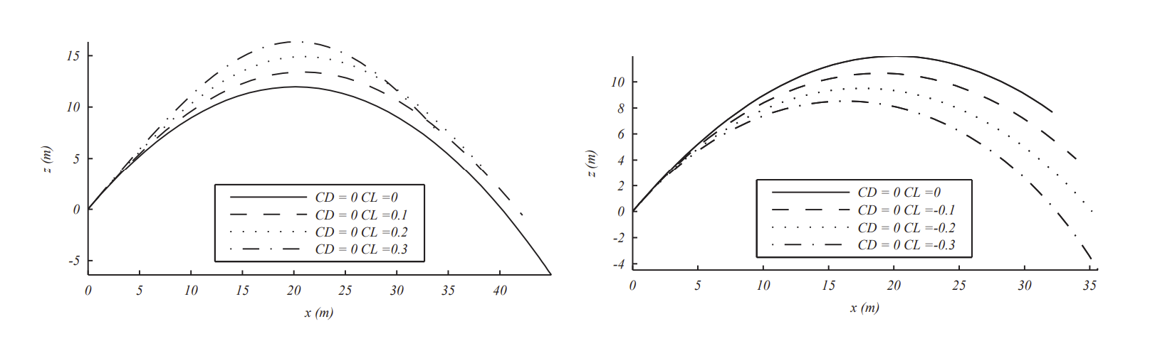
In Figures \(\PageIndex{3}\) and \(\PageIndex{4}\) we indicate what typical solutions would look like for different values of drag and lift coefficients. In the case of nonzero lift coefficients, we indicate positive and negative values leading to flight with top spin, \(C_{L}<0\), or bottom spin, \(C_{L}>0\).

Figure \(\PageIndex{4}\): Example of soccer ball under the influence of lift with \(C L>0\) and \(C L<0\)