3.5.4: Falling Raindrops

A SIMPLE PROBLEM THAT APPEARS IN MECHANICS is that of a falling raindrop through a mist. The raindrop not only undergoes free fall, but the mass of the drop grows as it interacts with the mist. There have been several papers written on this problem and it is a nice example to explore using numerical methods. In this section we look at models of a falling raindrop with and without air drag.

First we consider the case in which there is no air drag. A simple model of free fall from Newton’s Second Law of Motion is

\(\dfrac{d(m v)}{d t}=m g\)

In this discussion we will take downward as positive. Since the mass is not constant. we have

\(m \dfrac{d v}{d t}=m g-v \dfrac{d m}{d t}\)

In order to proceed, we need to specify the rate at which the mass is changing. There are several models one can adapt.We will borrow some of the ideas and in some cases the numerical values from Sokal(2010)\(^{1}\) and Edwards, Wilder, and Scime (2001).\(^{2}\) These papers also quote other interesting work on the topic.

1

A. D. Sokal, The falling raindrop, revisited, Am. J. Phys. 78, 643-645, (2010).

2

B. F. Edwards, J. W. Wilder, and E. E. Scime, Dynamics of Falling Raindrops, Eur. J. Phys. 22, 113-118, (2001).

While \(v\) and \(m\) are functions of time, one can look for a way to eliminate time by assuming the rate of change of mass is an explicit function of \(m\) and \(v\) alone. For example, Sokal (2010) assumes the form

\(\dfrac{d m}{d t}=\lambda m^{\sigma} v^{\beta}, \quad \lambda>0\)

This contains two commonly assumed models of accretion:

1. \(\sigma=2 / 3, \beta=0\). This corresponds to growth of the raindrop proportional to the surface area. Since \(m \propto r^{3}\) and \(A \propto r^{2}\), then \(m \propto A\) implies that \(\dot{m} \propto m^{2 / 3}\).
2. \(\sigma=2 / 3, \beta=1\). In this case the growth of the raindrop is proportional to the volume swept out along the path. Thus, \(\Delta m \propto A(v \Delta t)\), where \(A\) is the cross sectional area and \(v \Delta t\) is the distance traveled in time \(\Delta t\)

In both cases, the limiting value of the acceleration is a constant. It is \(g / 4\) in the first case and \(g / 7\) in the second case.

Another approach might be to use the effective radius of the drop, assuming that the raindrop remains close to spherical during the fall. According to Edwards, Wilder, and Scime (2001), raindrops with Reynolds number greater than 1000 and with radii larger than i mm will flatten. Even larger raindrops will break up when the drag force exceeds the surface tension. Therefore, they take \(0.1 \mathrm{~mm}<r<1 \mathrm{~mm}\) and \(10<R e<1000\). We will return to a discussion of the drag later.

It might seem more natural to make the radius the dynamic variable, than the mass. In this case, we can assume the accretion rate takes the form

\(\dfrac{d r}{d t}=\gamma r^{\alpha} v^{\beta}, \quad \gamma>0\)

Since, \(m=\dfrac{4}{3} \pi \rho_{d} r^{3}\)

\(\dfrac{d m}{d t} \sim r^{2} \dfrac{d r}{d t} \sim m^{2 / 3} \dfrac{d r}{d t}\)

Therefore, the two special cases become

1. \(\alpha=0, \beta=0\). This corresponds to a growth of the raindrop proportional to the surface area.
2. \(\alpha=0, \beta=1\). In this case the growth of the raindrop is proportional to the volume swept out along the path.

Here \(\rho_{d}\) is the density of the raindrop. We will also need

\[\begin{aligned} \dfrac{v}{m} \dfrac{d m}{d t} &=\dfrac{4 \pi \rho_{d} r^{2}}{\dfrac{4}{3} \pi \rho_{d} r^{3}} v \dfrac{d r}{d t} \\ &=3 \dfrac{v}{r} \dfrac{d r}{d t} \\ &=3 \gamma r^{\alpha-1} v^{\beta+1} \end{aligned} \label{3.39} \]

Putting this all together, we have a systems of two equations for \(v(t)\) and \(r(t)\) :

\[\begin{aligned} \dfrac{d v}{d t} &=g-3 \gamma r^{\alpha-1} v^{\beta+1} \\ \dfrac{d r}{d t} &=\gamma r^{\alpha} v^{\beta} \end{aligned}\label{3.40} \]

Example \(\PageIndex{1}\)

Determine \(v=v(r)\) for the case \(\alpha=0, \beta=0\) and the initial conditions \(r(0)=0.1 \mathrm{~mm}\) and \(v(0)=0 \mathrm{~m} / \mathrm{s}\).

In this case Equations \(\PageIndex{2}\) become

\[ \begin{aligned} &\dfrac{d v}{d t}=g-3 \gamma r^{-1} v \\ &\dfrac{d r}{d t}=\gamma \end{aligned} \end{equation}\label{3.41} \]

Noting that

\[\dfrac{d v}{d t}=\dfrac{d v}{d r} \dfrac{d r}{d t}=\gamma \dfrac{d v}{d r}\nonumber \]

we can convert the problem to one of finding the solution \(v(r)\) subject to the equation

\[\dfrac{d v}{d r}=\dfrac{g}{\gamma}-3 \dfrac{v}{r}\nonumber \]

with the initial condition \(v\left(r_{0}\right)=0 \mathrm{~m} / \mathrm{s}\) for \(r_{0}=0.0001 \mathrm{~m}\).

Rearranging the differential equation, we find that it is a linear first order differential equation,

\[\dfrac{d v}{d r}+\dfrac{3}{r} v=\dfrac{g}{\gamma}\nonumber \]

This equation can be solved using an integrating factor, \(\mu=r^{3}\), obtaining

\[\dfrac{d}{d r}\left(r^{3} v\right)=\dfrac{g}{\gamma} r^{3}\nonumber \]

Integrating, we obtain the solution

\[v(r)=\dfrac{g}{4 \gamma} r\left(1-\left(\dfrac{r_{0}}{r}\right)^{4}\right)\nonumber \]

Note that for large \(r, v \sim \dfrac{g}{4 \gamma} r .\) Therefore, \(\dfrac{d v}{d t} \sim \dfrac{g}{4} .\)

While this case was easily solved in terms of elementary operations, it is not always easy to generate solutions to Equations \(\PageIndex{2}\) analytically. Sokal (2010) derived a general solution in terms of incomplete Beta functions, though this does not help visualize the solution. Also, as we will see, adding air drag will lead to a nonintegrable system. So, we turn to numerical solutions.

In MATLAB, we can use the function in raindropf.m to capture the system \(\PageIndex{2}). Here we put the velocity in \(y(1)\) and the radius in \(y(2)\).

function dy=raindropf(t,y);

global alpha beta gamma g

dy=[g-3*gamma*y(2)^(alpha-1)*y(1)^(beta+1); ...

gamma*y(2)^alpha*y(1)^beta];

We then use the Runge-Kutta solver, ode45, to solve the system. An implementation is shown below which calls the function containing the system. The value \(\gamma=2.5 \times 10^{-7}\) is based on empirical results quoted by Edwards, Wilder, and Scime (2001).

Figure \(\PageIndex{1}\): The plots of position and velocity as a function of time for \(\alpha=\beta=0\).

clear

global alpha beta gamma g

alpha=0;

beta=0;

gamma=2.5e-07;

g=9.81;

r0=0.0001;

v0=0;

y0=[v0;r0];

tspan=[0 1000];

[t,y]=ode45(@raindropf,tspan,y0);

plot(1000*y(:,2),y(:,1),’k’)

Figure \(\PageIndex{2}\): The plot the velocity as a function of position for \(\alpha=\beta=0\).

Figure \(\PageIndex{3}\): The plot the velocity as a function of position for \(\alpha=0, \beta=1\).

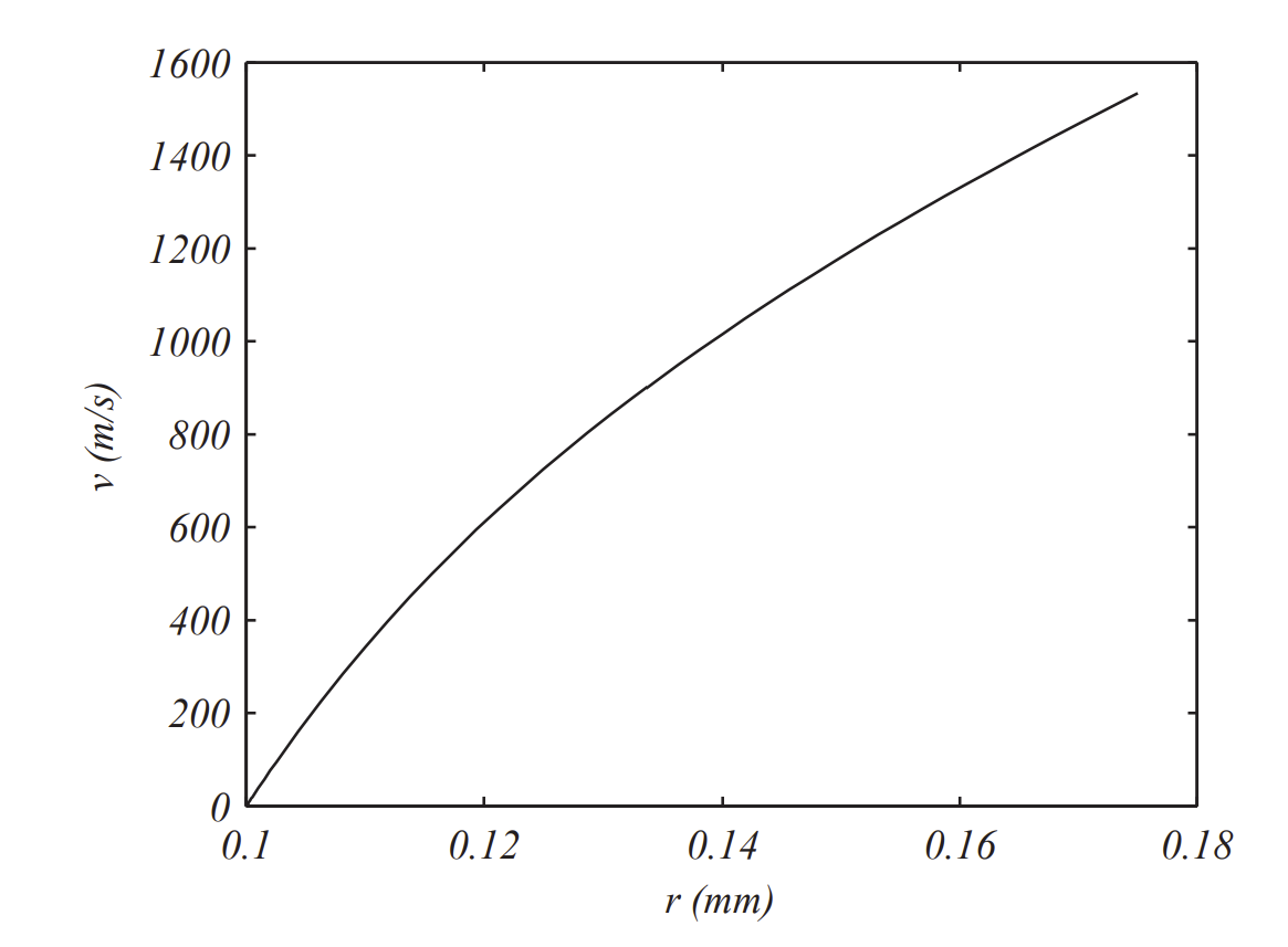
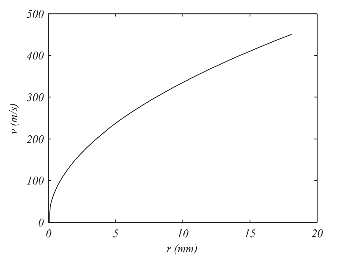
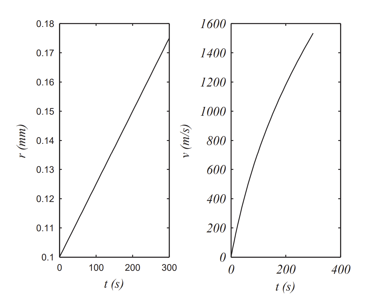
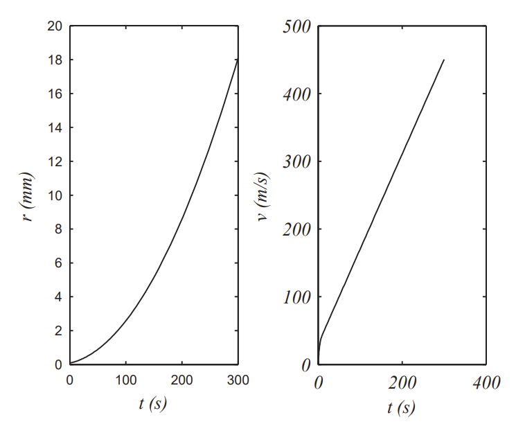
The resulting plots are shown in Figures \(\PageIndex{1}\)-\(\PageIndex{2}\). The plot of velocity as a function of position agrees with the exact solution, which we derived in the last example. We note that these drops do not grow much, but they seem to obtain large speeds.

For the second case, \(\alpha=0, \beta=1\), one can also obtain an exact solution. The result is

\[v(r)=\left[\dfrac{2 g}{7 \gamma} r\left(1-\left(\dfrac{r_{0}}{r}\right)^{7}\right)\right]^{\dfrac{1}{2}}\nonumber \]

For large \(r\) one can show that \(\dfrac{d v}{d t} \sim \dfrac{g}{7}\). In Figures \(3 \cdot 33^{-3} \cdot 3^{2}\) we see again large velocities, though about a third as fast over the same time interval. However, we also see that the raindrop has significantly grown well past the point it would break up.

In this simple model of a falling raindrop we have not considered air drag. Earlier in the chapter we discussed the free fall of a body with air resistance and this lead to a terminal velocity. Recall that the drag force given by

\[f_{D}(v)=-\dfrac{1}{2} C_{D} A \rho_{a} v^{2} \nonumber \]

where \(C_{D}\) is the drag coefficient, \(A\) is the cross sectional area and \(\rho_{a}\) is the air density. Also, we assume that the body is falling downward and downward is positive, so that \(f_{D}(v)<0\) so as to oppose the motion.

We would like to incorporate this force into our model \(\PageIndex{2}\). The first equation came from the force law, which now becomes

\[m \dfrac{d v}{d t}=m g-v \dfrac{d m}{d t}-\dfrac{1}{2} C_{D} A \rho_{a} v^{2}\nonumber \]

Or

\[\dfrac{d v}{d t}=g-\dfrac{v}{m} \dfrac{d m}{d t}-\dfrac{1}{2 m} C_{D} A \rho_{a} v^{2}\nonumber \]

The next step is to eliminate the dependence on the mass, \(m\), in favor of the radius, \(r\). The drag force term can be written as

\[ \begin{aligned} \dfrac{f_{D}}{m} &=\dfrac{1}{2 m} C_{D} A \rho_{a} v^{2} \\ &=\dfrac{1}{2} C_{D} \dfrac{\pi r^{2}}{\dfrac{4}{3} \pi \rho_{d} r^{3}} \rho_{a} v^{2} \\ &=\dfrac{3}{8} \dfrac{\rho_{a}}{\rho_{d}} C_{D} \dfrac{v^{2}}{r} \end{aligned} \label{3.43} \]

We had already done this for the second term; however, Edwards, Wilder, and Scime (2001) point to experimental data and propose that

\[\dfrac{d m}{d t}=\pi \rho_{m} r^{2} v \nonumber \]

where \(\rho_{m}\) is the mist density. So, the second terms leads to

\[\dfrac{v}{m} \dfrac{d m}{d t}=\dfrac{3}{4} \dfrac{\rho_{m}}{\rho_{d}} \dfrac{v^{2}}{r}\nonumber \]

Figure \(\PageIndex{4}\): The plots of position and velocity as a function of time for \(\alpha=0, \beta=\)

But, since \(m=\dfrac{4}{3} \pi \rho_{d} r^{3}\)

\[\dfrac{d m}{d t}=4 \pi \rho_{d} r^{2} \dfrac{d r}{d t}\nonumber \]

\(\mathrm{SO}\),

\[\dfrac{d r}{d t}=\dfrac{\rho_{m}}{4 \rho_{d}} v\nonumber \]

This suggests that their model corresponds to \(\alpha=0, \beta=1\), and \(\gamma=\dfrac{\rho_{m}}{4 \rho_{d}}\).

Now we can write down the modified system

\[\begin{aligned} \dfrac{d v}{d t} &=g-3 \gamma r^{\alpha-1} v^{\beta+1}-\dfrac{3}{8} \dfrac{\rho_{a}}{\rho_{d}} C_{D} \dfrac{v^{2}}{r} \\ \dfrac{d r}{d t} &=\gamma r^{\alpha} v^{\beta} \end{aligned} \label{3.44} \]

Edwards, Wilder, and Scime (2001) assume that the densities are constant with values \(\rho_{a}=.856 \mathrm{~kg} / \mathrm{m}^{3}, \rho_{d}=1.000 \mathrm{~kg} / \mathrm{m}^{3}\), and \(\rho_{m}=1.00 \times 10^{-3}\) \(\mathrm{kg} / \mathrm{m}^{3}\). However, the drag coefficient is not constant. As described later in Section 3.5.7, there are various models indicating the dependence of \(C_{D}\) on the Reynolds number,

\[R e=\dfrac{2 r v}{v}\nonumber \]

where \(v\) is the kinematic viscosity, which Edwards, Wilder, and Scime (2001) set to \(v=2.06 \times 10^{-5} \mathrm{~m}^{2} / \mathrm{s}\). For raindrops of the range \(r=0.1 \mathrm{~mm}\) to 1 \(\mathrm{mm}\), the Reynolds number is below rooo. Edwards, Wilder, and Scime (2001) modeled \(C_{D}=12 R e^{-1 / 2} .\) In the plots in Section \(3.5.7\) we include this model and see that this is a good approximation for these raindrops. In Chapter 10 we discuss least squares curve fitting and using these methods, one can use the models of Putnam (1961) and Schiller-Naumann (1933) to obtain a power law fit similar to that used here. So, introducing

\[C_{D}=12 R e^{-1 / 2}=12\left(\dfrac{2 r v}{v}\right)^{-1 / 2}\nonumber \]

and defining

\[\delta=\dfrac{9}{2^{3 / 2}} \dfrac{\rho_{a}}{\rho_{d}} v^{1 / 2}\nonumber \]

we can write the system of equations \(\PageIndex{6}\) as

\[\begin{aligned} \dfrac{d v}{d t} &=g-3 \gamma \dfrac{v^{2}}{r}-\delta\left(\dfrac{v}{r}\right)^{\dfrac{3}{2}} \\ \dfrac{d r}{d t} &=\gamma v . \end{aligned}\label{3.45} \]

Now, we can modify the MATLAB code for the raindrop by adding the extra term to the first equation, setting \(\alpha=0, \beta=1\), and using \(\delta=0.0124\) and \(\gamma=2.5 \times 10^{-7}\) from Edwards, Wilder, and Scime \((2001)\).

Figure \(\PageIndex{5}\): The plots of position and velocity as a function of time with air drag included.

Figure \(\PageIndex{6}\): The plot the velocity as a function of position with air drag included.

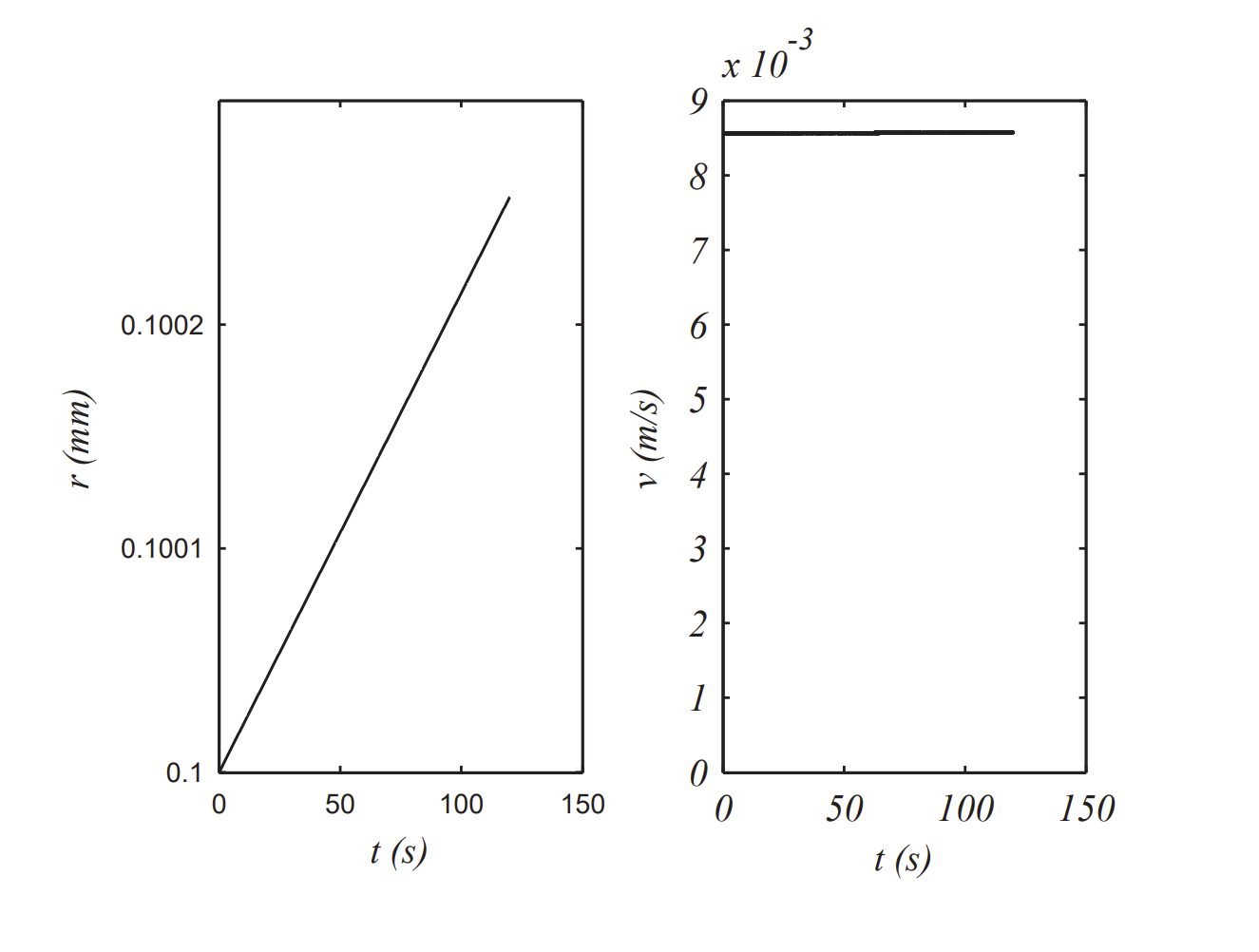
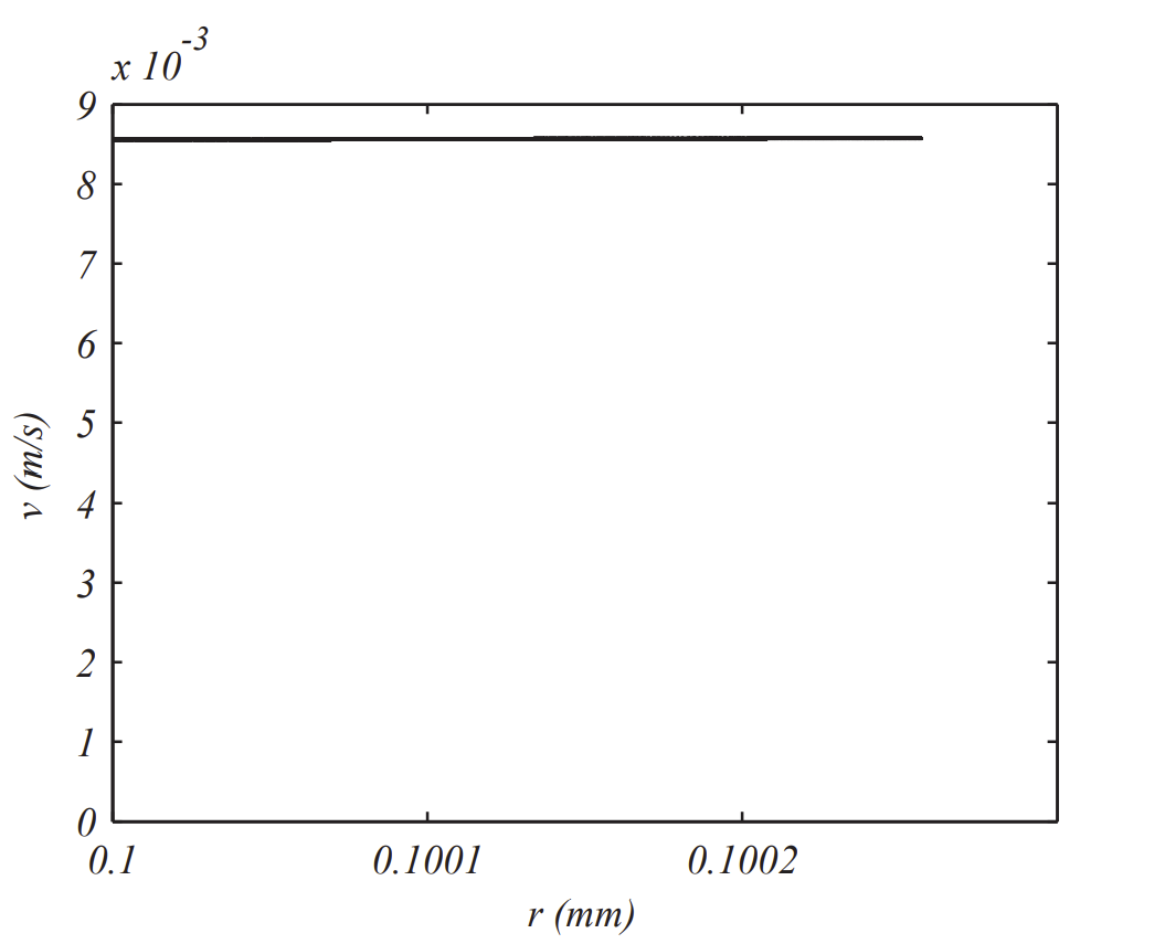
In Figures \(\PageIndex{5}\)- \(\PageIndex{6}\) we see different behaviors as compared to the previous models. It appears that the velocity quickly reaches a terminal velocity and the radius continues to grow linearly in time, though at a slow rate.

We might be able to understand this behavior. Terminal, or constant \(v\),

\[g-3 \gamma \dfrac{v^{2}}{r}-\delta\left(\dfrac{v}{r}\right)^{\dfrac{3}{2}}=0 \nonumber \]

Looking at these terms, one finds that the second term is significantly smaller

\[\delta\left(\dfrac{v}{r}\right)^{\dfrac{3}{2}} \approx g\nonumber \]

\[\dfrac{v}{r} \approx\left(\dfrac{g}{\delta}\right)^{2 / 3} \approx 85.54 \mathrm{~s}^{-1} \nonumber \]

This agrees with the numerical data which gives the slope of the \(v\) vs \(r\) plot would occur when than the other terms and thus

Or as \(85.5236 \mathrm{~s}^{-1}\).