3.5.1: The Nonlinear Pendulum

NOW WE WILL INVESTIGATE THE USE OF NUMERCIAL METHODS fOr SOLVing the nonlinear pendulum problem.

Example \(\PageIndex{1}\): Nonlinear Pendulum

Solve

\(\ddot{\theta}=-\dfrac{g}{L} \sin \theta, \quad \theta(0)=\theta_{0}, \quad \omega(0)=0, \quad t \in[0,8],\)

using Euler’s Method. Use the parameter values of \(m=0.005 \mathrm{~kg}\), \(L=0.500 \mathrm{~m}\), and \(g=9.8 \mathrm{~m} / \mathrm{s}^{2}\).

This is a second order differential equation. As describe later, we can write this differential equation as a system of two first order differential equations,

\[ \begin{equation}\begin{aligned} \dot{\theta} &=\omega, \\ \dot{\omega} &=-\dfrac{g}{L} \sin \theta . \end{aligned}\label{3.26} \]

Defining the vector

\( \Theta (t)=\left(\begin{array}{c} \theta(t) \\ \omega(t) \end{array}\right)\)

we can write the first order system as

\(\dfrac{d \Theta}{d t}=\mathbf{F}(t, \Theta), \quad \Theta(0)=\left(\begin{array}{c}
\theta_{0} \\
0
\end{array}\right)\)

where

\(F(t, \Theta)=\left(\begin{array}{c} \omega(t) \\ -\dfrac{g}{L} \sin \theta(t) \end{array}\right)\)

This allows us to use the the methods we have discussed on this first order equation for \(\Theta(t)\).

For example, Euler’s Method for this system becomes

\(\Theta_{i+1}=\Theta_{i+1}+h \mathbf{F}\left(t_{i}, \Theta_{i}\right)\)

With \(\Theta_{0}=\Theta(0)\).

We can write this scheme in component form as

\(\left(\begin{array}{c} \theta_{i+1} \\ \omega_{i+1} \end{array}\right)=\left(\begin{array}{c} \theta_{i} \\ \omega_{i} \end{array}\right)+h\left(\begin{array}{c} \omega_{i} \\ -\dfrac{g}{L} \sin \theta_{i} \end{array}\right)\)

or

\[ \begin{aligned} \theta_{i+1} &=\theta_{i}+h \omega_{i} \\ \omega_{i+1} &=\omega_{i}-h \dfrac{g}{L} \sin \theta_{i} \end{aligned}\label{3.27} \]

starting with \(\theta_{0}=\theta_{0}\) and \(\omega_{0}=0\).

The MATLAB code that can be used to implement this scheme takes the form.

g=9.8;

L=0.5;

m=0.005;

a=0;

b=8;

N=500;

h=(b-a)/N;

% Initial Condition

t(1)=0;

theta(1)=pi/6;

omega(1)=0;

% Euler’s Method for

i=2:N+1

omega(i)=omega(i-1)-g/L*h*sin(theta(i-1));

theta(i)=theta(i-1)+h*omega(i-1);

t(i)=t(i-1)+h;

end

Figure \(\PageIndex{1}\): Solution for the nonlinear pendulum problem using Euler’s Method on \(t \in[0,8]\) with \(N=500\).

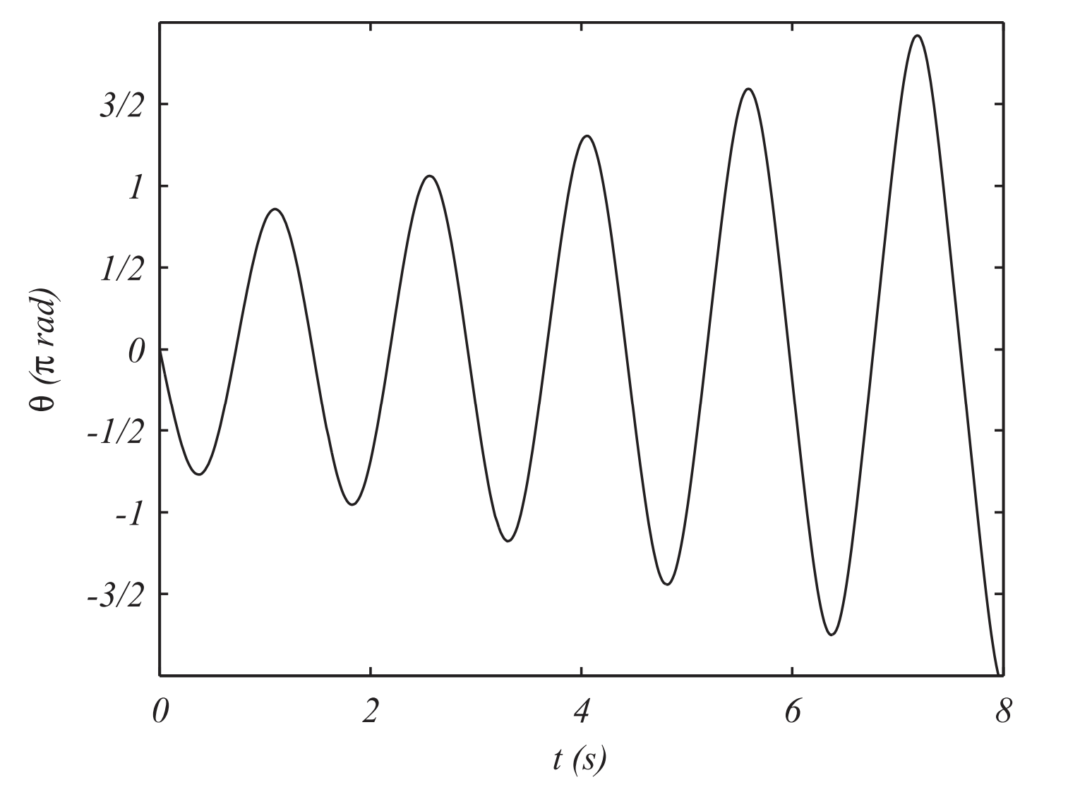
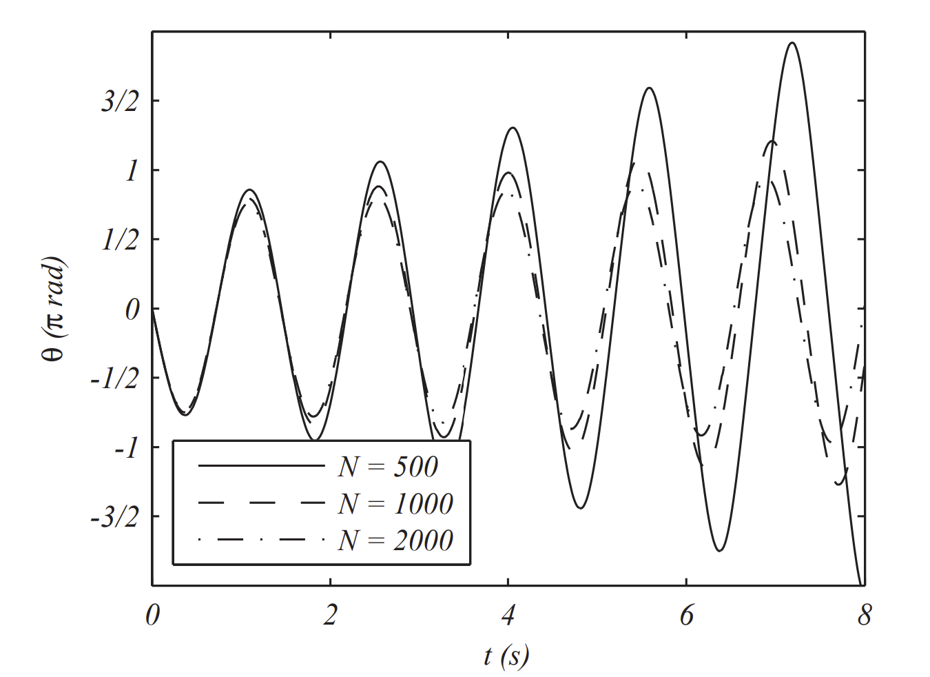
In Figure \(\PageIndex{1}\) we plot the solution for a starting position of \(30^{0}\) with \(N = 500\). Notice that the amplitude of oscillation is increasing, contrary to our experience. So, we increase N and see if that helps. In Figure \(\PageIndex{2}\) we show the results for \(N =\) 500, 1000, and 2000 points, or \(h = \)0.016, 0.008, and 0.004, respectively. We note that the amplitude is not increasing as much.

The problem with the solution is that Euler’s Method is not an energy conserving method. As conservation of energy is important in physics, we would like to be able to seek problems which conserve energy. Such schemes used to solve oscillatory problems in classical mechanics are called symplectic integrators. A simple example is the Euler-Cromer, or semi-implicit Euler Method. We only need to make a small modification of Euler’s Method. Namely, in the second equation of the method we use the updated value of the dependent variable as computed in the first line.

Figure \(\PageIndex{2}\): Solution for the nonlinear pendulum problem using Euler’s Method on \(t \in[0,8]\) with \(N= 500,1000,2000\).

Let’s write the Euler scheme as

\[ \begin{aligned} \omega_{i+1}=\omega_{i}-h \dfrac{g}{L} \sin \theta_{i} \\ \theta_{i+1}=\theta_{i}+h \omega_{i} \end{aligned}\label{3.28} \]

Then, we replace \(\omega_{i}\) in the second line by \(\omega_{i+1}\) to obtain the new scheme

\[ \begin{aligned} \omega_{i+1} &=\omega_{i}-h \dfrac{g}{L} \sin \theta_{i} \\ \theta_{i+1} &=\theta_{i}+h \omega_{i+1} \end{aligned} \label{3.29} \]

The MATLAB code is easily changed as shown below.

g=9.8;

L=0.5;

m=0.005;

a=0;

b=8;

N=500;

h=(b-a)/N;

% Initial Condition

t(1)=0;

theta(1)=pi/6;

omega(1)=0;

% Euler-Cromer Method

for i=2:N+1

omega(i)=omega(i-1)-g/L*h*sin(theta(i-1));

theta(i)=theta(i-1)+h*omega(i);

t(i)=t(i-1)+h;

end

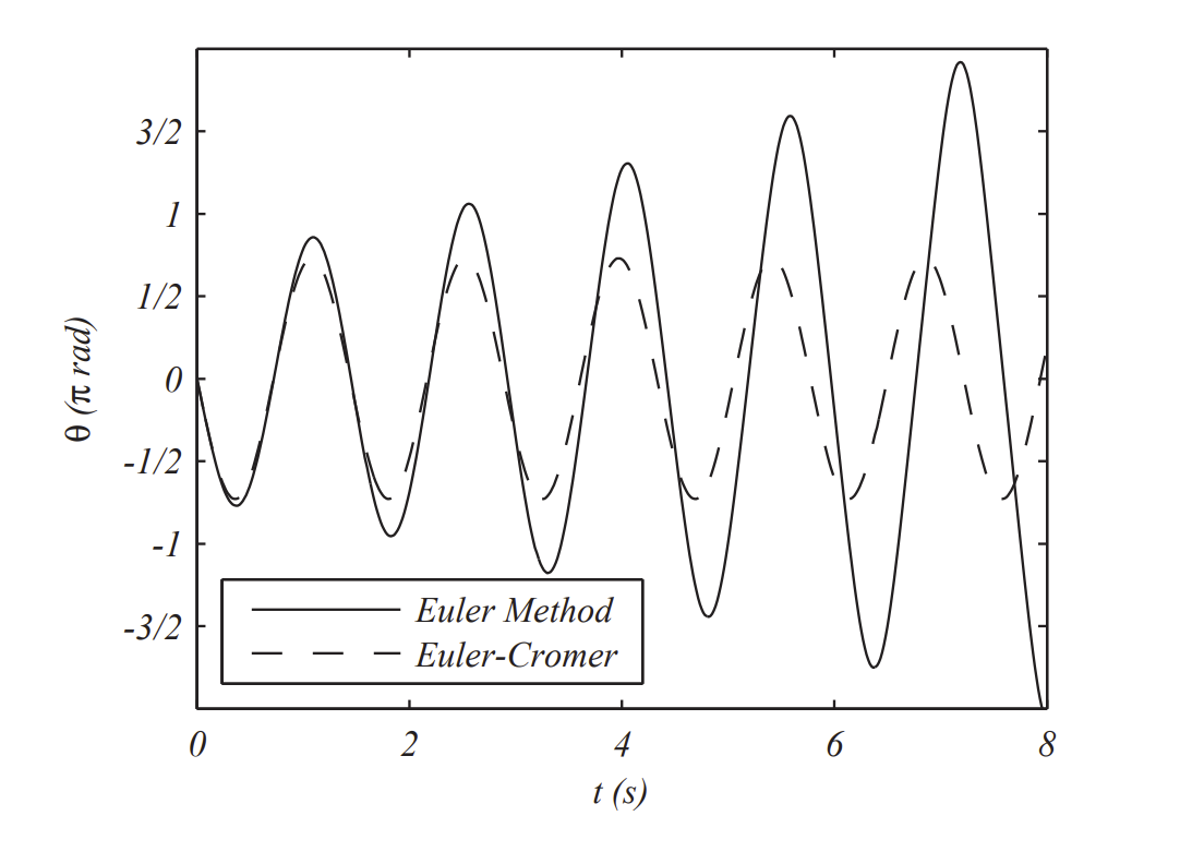
We then run the new scheme for \(N=500\) and compare this with what we obtained before. The results are shown in Figure \(\PageIndex{3}\). We see that the oscillation amplitude seems to be under control. However, the best test would be to investigate if the energy is conserved.

Recall that the total mechanical energy for a pendulum consists of the kinetic and gravitational potential energies,

\(E=\dfrac{1}{2} m v^{2}+m g h\)

For the pendulum the tangential velocity is given by \(v=L \omega\) and the height of the pendulum mass from the lowest point of the swing is \(h=L(1-\cos \theta)\). Therefore, in terms of the dynamical variables, we have

\[E=\dfrac{1}{2} m L^{2} \omega^{2}+m g L(1-\cos \theta) \nonumber \]

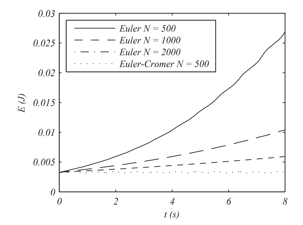
We can compute the energy at each time step in the numerical simulation. In MATLAB it is easy to do using

E = 1/2*m*L^2*omega.^2+m*g*L*(1-cos(theta));

after implementing the scheme. In other programming environments one needs to loop through the times steps and compute the energy along the way. In Figure \(\PageIndex{4}\) we shown the results for Euler’s Method for \(N=\) \(500,1000,2000\) and the Euler-Cromer Method for \(N=500\). It is clear that the Euler-Cromer Method does a much better job at maintaining energy conservation.

Figure \(\PageIndex{3}\): Solution for the nonlinear pendulum problem comparing Euler’s Method and the Euler-Cromer Method on \(t \in[0,8]\) with \(N=500\).

Figure \(\PageIndex{4}\): Total energy for the nonlinear pendulum problem.