3.5.5: The Two-body Problem

A STANDARD PROBLEM IN CLASSICAL DYNAMICS is the study of the motion of several bodies under the influence of Newton’s Law of Gravitation. The so-called \(n\)-body problem is not solvable. However, the two body problem is. Such problems can model the motion of a planet around the sun, the moon around the Earth, or a satellite around the Earth. Further interesting, and more realistic problems, would involve perturbations of these orbits due to additional bodies. For example, one can study problems such as the influence of large planets on the asteroid belt. Since there are no analytic solutions to these problems, we have to resort to finding numerical solutions. We will look at the two body problem since we can compare the

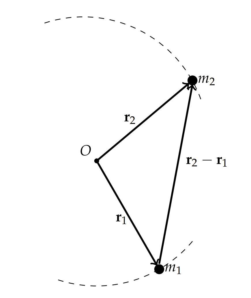
We consider two masses, \(m_{1}\) and \(m_{2}\), located at positions, \(\mathbf{r}_{1}\) and \(\mathbf{r}_{2}\), respectively, as shown in Figure \(3.36\). Newton’s Law of Gravitation for the force between two masses separated by position vector \(\mathbf{r}\) is given by

\[\mathbf{F}=-\dfrac{G m_{1} m_{2}}{r^{2}} \dfrac{\mathbf{r}}{r}\nonumber \]

Each mass experiences this force due to the other mass. This gives the system of equations

\[m_{1} \ddot{\mathbf{r}}_{1}=-\dfrac{G m_{1} m_{2}}{\left|\mathbf{r}_{2}-\mathbf{r}_{1}\right|^{3}}\left(\mathbf{r}_{1}-\mathbf{r}_{2}\right) \nonumber \]

\[m_{2} \ddot{\mathbf{r}}_{2}=-\dfrac{G m_{1} m_{2}}{\left|\mathbf{r}_{2}-\mathbf{r}_{1}\right|^{3}}\left(\mathbf{r}_{2}-\mathbf{r}_{1}\right) \nonumber \]

Now we seek to set up this system so that we can find numerical solutions for the positions of the masses. From the conservation of angular momentum, we know that the motion takes place in a plane. [Note: The solution of the Kepler Problem is discussed in Chapter 9.] We will choose the orbital plane to be the \(x y\)-plane. We define \(r_{12}=\left|\mathbf{r}_{2}-\mathbf{r}_{1}\right|\), and \(\left(x_{i}, y_{i}\right)=\mathbf{r}_{i}\), \(i=1,2 .\) Furthermore, we write the two second order equations as four first order equations. So, defining the velocity components as \(\left(u_{i}, v_{i}\right)=\mathbf{v}_{i}\), the system of equations can be written in the form

\[\dfrac{d}{d t}\left(\begin{array}{c} x_{1} \\ y_{1} \\ x_{2} \\ y_{2} \\ u_{1} \\ v_{1} \\ u_{2} \\ v_{2} \end{array}\right)=\left(\begin{array}{c} u_{1} \\ v_{1} \\ u_{2} \\ v_{2} \\ -\alpha m_{2}\left(x_{1}-x_{2}\right) \\ -\alpha m_{2}\left(y_{1}-y_{2}\right) \\ -\alpha m_{1}\left(x_{2}-x_{1}\right) \\ -\alpha m_{1}\left(y_{2}-y_{1}\right) \end{array}\right) \label{3.48} \]

Figure \(\PageIndex{1}\): Two masses interact under Newton’s Law of Gravitation. system of equations can be written in the form

Figure \(\PageIndex{2}\): Simulation of two bodies under gravitational attraction. function \(d z=\) twobody \((t, z)\)

function dz = twobody(t,z)

dz = zeros(8,1);

G = 1;

m1 = .1;

m2 = 2;

r=((z(1) - z(3)).^2 + (z(2) - z(4)).^2).^(3/2);

alpha=G/r;

dz(1) = z(5);

dz(2) = z(6);

dz(3) = z(7);

dz(4) = z(8);

dz(5) = alpha*m2*(z(3) - z(1));

dz(6) = alpha*m2*(z(4) - z(2));

dz(7) = alpha*m1*(z(1) - z(3));

dz(8) = alpha*m1*(z(2) - z(4));

In the above code we picked some seemingly nonphysical numbers for \(G\) and the masses. Calling ode 45 with a set of initial conditions,

[t,z] = ode45(’twobody’,[0 20], [-1 0 0 0 0 -1 0 0]);

plot(z(:,1),z(:,2),’k’,z(:,3),z(:,4),’k’);

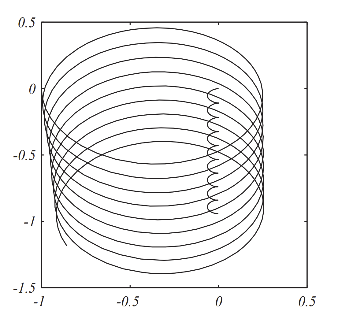
we obtain the plot shown in Figure \(\PageIndex{2}\). We see each mass moves along what looks like elliptical helices with the smaller body tracing out a larger orbit.

In the case of a very large body, most of the motion will be due to the smaller body. So, it might be better to plot the relative motion of the small body with respect to the larger body. Actually, an analysis of the two body problem shows that the center of mass

\[\mathbf{R}=\dfrac{m_{1} \mathbf{r}_{1}+m_{2} \mathbf{r}_{2}}{m_{1}+m_{2}}\nonumber \]

satisfies \(\ddot{\mathbf{R}}=0 .\) Therefore, the system moves with a constant velocity.

The relative position of the masses is defined through the variable \(\mathbf{r}=\) \(\mathbf{r}_{1}-\mathbf{r}_{2}\). Dividing the masses from the left hand side of Equations \(\PageIndex{2}\) and subtracting, we have the motion of \(m_{1}\) about \(m_{2}\)

\[\ddot{\mathbf{r}}=-G\left(m_{1}+m_{2}\right) \dfrac{\mathbf{r}}{r^{3}}\nonumber \]

where \(r=|\mathbf{r}|=\left|\mathbf{r}_{1}-\mathbf{r}_{2}\right| .\) Note that \(\mathbf{r} \times \ddot{\mathbf{r}}=0 .\) Integrating, this gives \(\mathbf{r} \times \dot{\mathbf{r}}=\) constant. This is just a statement of the conservation of angular momentum.

The orbiting body will remain in a plane and, therefore, we can take the \(z\)-axis perpendicular to \(\mathbf{r} \times \dot{\mathbf{r}}\), the position as \(\mathbf{r}=(x(t), y(t))\), and the velocity as \(\dot{\mathbf{r}}=(u(t), v(t)) .\) Then, the equations of motion can be written as four first order equations:

\[ \begin{aligned} &\dot{x}=u \\ &\dot{y}=v \end{aligned} \nonumber \]

\[\begin{aligned} \dot{u} &=-\mu \dfrac{x}{r^{3}} \\ \dot{v} &=-\mu \dfrac{y}{r^{3}} \end{aligned} \label{3.49} \]

where \(\mu=G\left(m_{1}+m_{2}\right)\) and \(r=\sqrt{x^{2}+y^{2}}\).

While we have established a system of equations which can be integrated, we should note a few results from the study of the Kepler problem in classical dynamics which we review in Chapter 9. Kepler’s Laws of Planetary Motion state:

1. All planets travel in ellipses.

The polar equation for the path is given by

\[r=\dfrac{a\left(1-e^{2}\right)}{1+e \cos \phi}\nonumber \]

where \(e\) is the eccentricity and \(a\) is the length of the semimajor axis. For \(0 \leq e<1\), the orbit is an ellipse.

2. A planet sweeps out equal areas in equal times.
3. The square of the period of the orbit is proportional to the cube of the semimajor axis. In particular, one can show that

\[T^{2}=\dfrac{4 \pi^{2}}{\mu} a^{3}\nonumber \]

By an appropriate choice of units, we can make \(\mu=G\left(m_{1}+m_{2}\right)\) a reasonable number. For the Earth-Sun system,

\[\begin{aligned} \mu &=6.67 \times 10^{-11} m^{3} k g^{-1} s^{-2}\left(1.99 \times 10^{30}+5.97 \times 10^{24}\right) k g \\ &=1.33 \times 10^{20} m^{3} s^{-1} \end{aligned} \nonumber \]

That is a large number and can cause problems in the numerics. However, if one uses astronomical scales, such as putting lengths in astronomical units, \(1 \mathrm{AU}=1.50 \times 10^{8} \mathrm{~km}\), and time in years, then

\[\mu=\dfrac{4 \pi^{2}}{T^{2}} a^{3}=4 \pi^{2}\nonumber \]

in units of \(A U^{3} / y r^{2}\).

Setting \(\phi=0\), the location of the perigee is given by

\[r=\dfrac{a\left(1-e^{2}\right)}{1+e}=a(1-e)\nonumber \]

or

\[\mathbf{r}=(a(1-e), 0)\nonumber \]

At this point the velocity is given by

\[\dot{\mathbf{r}}=\left(0, \sqrt{\dfrac{\mu}{a} \dfrac{1+e}{1-e}}\right) .\nonumber \]

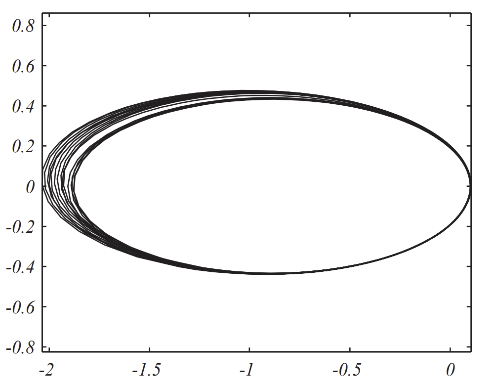
Knowing the position and velocity at \(\phi=0\), we can set the initial conditions for a bound orbit. The MATLAB code based on the above analysis is given below and the solution can be seen in Figure \(\PageIndex{3}\).

Figure \(\PageIndex{3}\): Simulation of one body orbiting a larger body under gravitational attraction

e=0.9;

tspan=[0 100];

z0=[1-e;0;0;sqrt((1+e)/(1-e))];

[t,z] = ode45(’twobodyf’,tspan, z0);

plot(z(:,1),z(:,2),’k’);

axis equal

function dz = twobodyf(t,z)

dz = zeros(4,1);

GM = 1;

r=(z(1).^2 + z(2).^2).^(3/2);

alpha=GM/r;

dz(1) = z(3);

dz(2) = z(4);

dz(3) = -alpha*z(1);

dz(4) = -alpha*z(2);

While it is clear that the mass is following an elliptical orbit, we see that it will only do so for a finite period of time partly because the RungeKutta code does not conserve energy and it does not conserve the angular momentum. The conservation of energy is found (up to a factor of \(m_{1}\) ) as

\[\dfrac{1}{2}\left(\dot{x}^{2}+\dot{y}^{2}\right)-\dfrac{\mu}{t}=-\dfrac{\mu}{2 a}\nonumber \]

Similarly, the conservation of (specific) angular momentum is given by

\[\mathbf{r} \times \mathbf{v}=(x \dot{y}-y \dot{x}) \mathbf{k}=\sqrt{\mu a\left(1-e^{2}\right)} \mathbf{k}\nonumber \]

As was the case with the nonlinear pendulum example, we saw that an implicit Euler method, or Cromer’s method, was better at conserving energy. So, we compare the Euler’s Method version with the Implicit-Euler Method. In general, we seek to solve the system

\[ \begin{aligned} \dot{\mathbf{r}} &=\mathbf{F}(\mathbf{r}, \mathbf{v}) \\ \dot{\mathbf{v}} &=\mathbf{G}(\mathbf{r}, \mathbf{v}) \end{aligned} \label{3.50} \]

As we had seen earlier, Euler’s Method is given by

\[ \begin{aligned} \mathbf{v}_{n} &=\mathbf{v}_{n-1}+\Delta t * \mathbf{G}\left(t_{n-1}, \mathbf{x}_{n-1}\right) \\ \mathbf{r}_{n} &=\mathbf{r}_{n-1}+\Delta t * \mathbf{F}\left(t_{n-1}, \mathbf{v}_{n-1}\right) \end{aligned} \label{3.51} \]

For the two body problem, we can write out the Euler Method steps using \(\mathbf{v}=(u, v), \mathbf{r}=(x, y), \mathbf{F}=(u, v)\), and \(\mathbf{G}=-\dfrac{\mu}{r^{3}}(x, y) .\) (Euler’s Method for the two body problem)The MATLAB code would use the loop

for i=2:N+1

alpha=mu/(x(i-1).^2 + y(i-1).^2).^(3/2);

u(i)=u(i-1)-h*alpha*x(i-1);

v(i)=v(i-1)-h*alpha*y(i-1);

x(i)=x(i-1)+h*u(i-1);

y(i)=y(i-1)+h*v(i-1);

t(i)=t(i-1)+h;

end

Note that more compact forms can be used, but they are not readily adaptable to other packages or programming languages.

Figure \(\PageIndex{4}\): Results for using Euler method for \(N = 4000000\) and \(t \in [0, 100]\). The parameters are \(\mu = 1\), \(e = 0, 9\), and \(a = 1\).

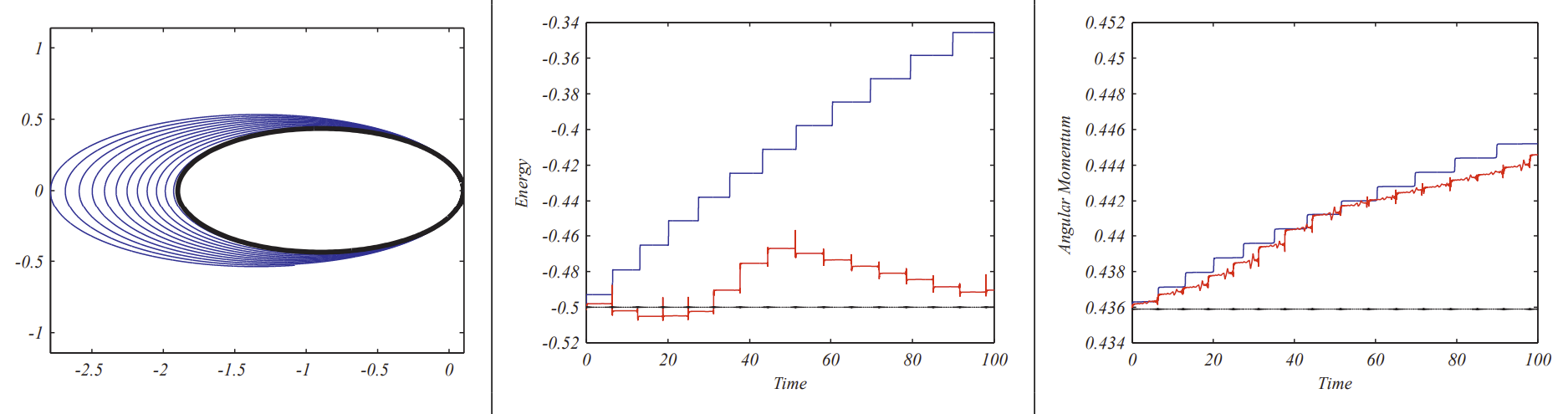
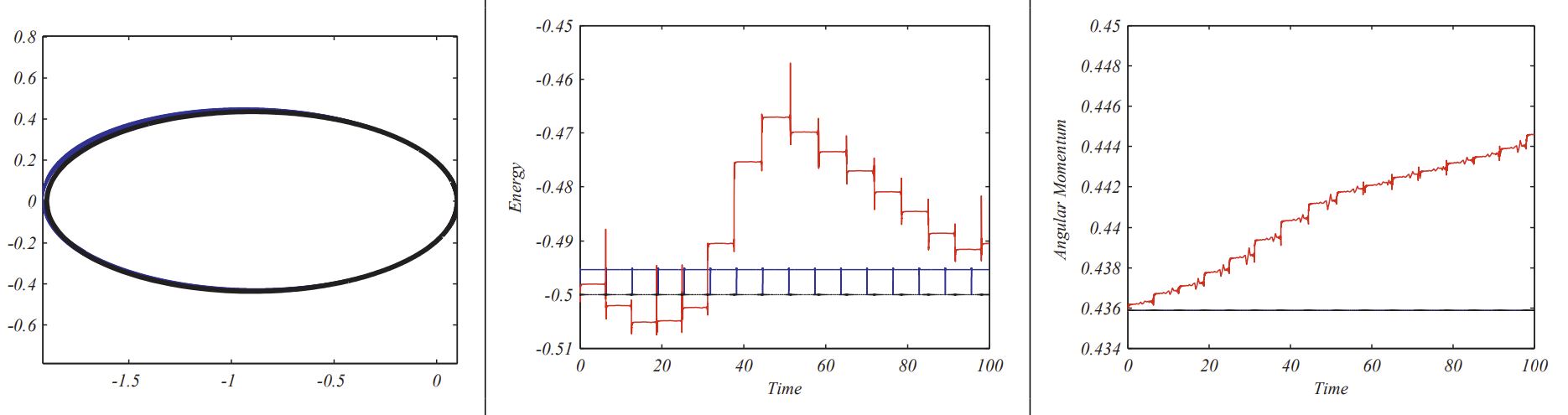
In Figure \(3.8\) we show the results along with the energy and angular momentum plots for \(N=4000000\) and \(t \in[0,100]\) for the case of \(\mu=1\), The par \(a=1\). \(e=0,9\), and \(a=1\). The orbit based on the exact solution is in the center of the figure on the left. The energy and angular momentum as a function of time are shown along with the similar plots obtained using ode 45 . In neither case are these two quantities conserved.

for i=2:N+1

alpha=mu/(x(i-1).^2 + y(i-1).^2).^(3/2);

u(i)=u(i-1)-h*alpha*x(i-1);

v(i)=v(i-1)-h*alpha*y(i-1);

x(i)=x(i-1)+h*u(i);

y(i)=y(i-1)+h*v(i);

t(i)=t(i-1)+h;

end

(Implicit-Euler Method for the two body)The Implicit-Euler Method is a slight modification to the Euler Method problem and has a better chance at handing the conserved quantities as the ImplicitEuler Method is one of many symplectic integrators. The modification uses the new value of the velocities in the updating of the position. Thus, we have

\[ \begin{array}{r} \mathbf{v}_{n}=\mathbf{v}_{n-1}+\Delta t * \mathbf{G}\left(t_{n-1}, \mathbf{x}_{n-1}\right) \\ \mathbf{r}_{n}=\mathbf{r}_{n-1}+\Delta t * \mathbf{F}\left(t_{n-1}, \mathbf{v}_{n}\right) \end{array} \label{3.52} \]

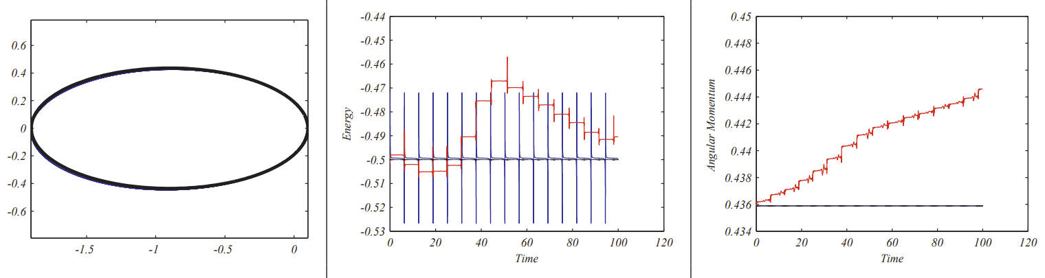
It is a simple matter to update the MATLAB code. In Figure \(3.9\) we show the results along with the energy and angular momentum plots for \(N=\) 200000 and \(t \in[0,100]\) for the case of \(\mu=1, e=0,9\), and \(a=1\). The orbit based on the exact solution coincides with the orbit as seen in the left figure. The energy and angular momentum as functions of time are appear to be conserved. The energy fluctuates about \(-0.5\) and the angular momentum remains constant. Again, the ode45 results are shown in comparison. The number of time steps has been decreased from the Euler Method by a factor of 20 .

Figure \(\PageIndex{5}\): Results for using the ImplicitEuler method for \(N=200000\) and \(t \in\) \([0,100]\). The parameters are \(\mu=1, e=\) 0,9 , and \(a=1\).

The Euler and Implicit Euler are first order methods. We can attempt a faster and more accurate process which is also a symplectic method. As a final example, we introduce the velocity Verlet method for solving

\[\ddot{\mathbf{r}}=\mathbf{a}(\mathbf{r}(t)) \nonumber \]

The derivation is based on a simple Taylor expansion:

\[\mathbf{r}(t+\Delta t)=\mathbf{r}(t)+\mathbf{v}(t) \Delta t+\dfrac{1}{2} \mathbf{a}(\mathbf{t}) \Delta t^{2}+\cdots \cdot\nonumber \]

Replace \(\Delta t\) with \(-\Delta t\) to obtain

\[\mathbf{r}(t-\Delta t)=\mathbf{r}(t)-\mathbf{v}(t) \Delta t+\dfrac{1}{2} \mathbf{a}(\mathbf{t}) \Delta t^{2}-\cdots \cdot\nonumber \]

Now, adding these expressions leads to some cancellations,

\[\mathbf{r}(t+\Delta t)=2 \mathbf{r}(t)-\mathbf{r}(t-\Delta t)+\mathbf{a}(\mathbf{t}) \Delta t^{2}+O\left(\Delta t^{4}\right)\nonumber \]

Writing this in a more useful form, we have

\[\mathbf{r}_{n+1}=2 \mathbf{r}_{n}-\mathbf{r}_{n-1}+\mathbf{a}\left(\mathbf{r}_{n}\right) \Delta t^{2}\nonumber \]

Thus, we can find \(\mathbf{r}_{n+1}\) from the previous two values without knowing the velocity. This method is called the Verlet, or Störmer-Verlet Method.

Loup Verlet (1931-) is a physicist who works on molecular dynamics and Fredrik Carl Mülertz Störmer (1874-1957) was a mathematician and physicist who modeled the motion of charged particles in his studies of the aurora borealis.

It is useful to know the velocity so that we can check energy conservation and angular momentum conservation. The Verlet Method can be rewritten in the Stömer-Verlet Method in an equivalent form know as the velocity Verlet method. We use

\[\mathbf{r}(t)-\mathbf{r}(t-\Delta t) \approx \mathbf{v}(t) \Delta t-\dfrac{1}{2} \mathbf{a} \Delta t^{2} \nonumber \]

in the Stömer-Verlet Method and write

\[ \begin{aligned} \mathbf{r}_{n} &=\mathbf{r}_{n-1}+\mathbf{v}_{n-1} u+\dfrac{h^{2}}{2} \mathbf{a}\left(\mathbf{r}_{n-1}\right), \\ \mathbf{v}_{n-1 / 2} &=\mathbf{v}_{n-1}+\dfrac{h}{2} \mathbf{a}\left(\mathbf{r}_{n-1}\right), \\ \mathbf{a}_{n} &=\mathbf{a}\left(\mathbf{r}_{n}\right), \\ \mathbf{v}_{n} &=\mathbf{v}_{n-1 / 2}+\dfrac{h}{2} \mathbf{a}_{n}, \end{aligned}\label{3.53} \]

where \(h=\Delta t .\) For the current problem, \(\mathbf{a}\left(\mathbf{r}_{n}\right)=-\dfrac{\mu}{r_{n}^{2}} \mathbf{r}_{n} .\)

(Störmer-Verlet Method for the two body problem.)

The MATLAB snippet is given as

for i=2:N+1

alpha=mu/(x(i-1).^2 + y(i-1).^2).^(3/2);

x(i)=x(i-1)+h*u(i-1)-h^2/2*alpha*x(i-1);

y(i)=y(i-1)+h*v(i-1)-h^2/2*alpha*y(i-1);

u(i)=u(i-1)-h/2*alpha*x(i-1);

v(i)=v(i-1)-h/2*alpha*y(i-1);

alpha=mu/(x(i).^2 + y(i).^2).^(3/2);

u(i)=u(i)-h/2*alpha*x(i);

v(i)=v(i)-h/2*alpha*y(i);

t(i)=t(i-1)+h;

end

The results using the velocity Verlet method are shown in Figure \(\PageIndex{6}\). For only 50,000 steps we have
and the orbit appears stable.

Figure \(\PageIndex{6}\): Results for using velocity Verlet method for \(N = 50000\) and \(t \in [0, 100]\). The parameters are \(\mu = 1\), \(e = 0, 9\), and \(a = 1\).