3.5.6: The Expanding Universe
- Page ID
- 103784

ONE OF THE REMARKABLE STORIES Of the twentieth century is the development of both the theory and the experimental data leading to our current understanding of the large scale structure of the universe. In 1916 Albert Einstein (1879-1955) published his general theory of relativity. It is a geometric theory of gravitation which relates the curvature of spacetime to its energy and momentum content. This relationship is embodied in the Einstein field equations, which are written compactly as
\[G_{\mu v}+\Lambda g_{\mu v}=\dfrac{8 \pi G}{c^{4}} T_{\mu v}\nonumber \]
The left side contains the curvature of spacetime as determined by the metric \(g_{\mu v}\). The Einstein tensor, \(G_{\mu v}=R_{\mu v}-\dfrac{1}{2} R g_{\mu v}\), is determined from the curvature tensor \(R_{\mu v}\) and the scalar curvature, \(R\). These in turn are obtained from the metric tensor. \(\Lambda\) is the famous cosmological constant, which Einstein originally introduced to maintain a static universe, which has since taken on a different role. The right-hand side of Einstein’s equation involves the familiar gravitational constant, the speed of light, and the stress-energy tensor, \(T_{\mu v}\).
Georges Lemaitre (1894-1966) had actually predicted the expansion of the universe in 1927 and proposed what later became known as the big bang theory.
In 1917 Einstein applied general relativity to cosmology. However, it was Alexander Alexandrovich Friedmann (1888-1925) who was the first to provide solutions to Einstein’s equation based on the assumptions of homogeneity and isotropy and leading to the expansion of the universe. Unfortunately, Friedmann died in 1925 of typhoid.
In 1929 Edwin Hubble (1889-1953) showed that the radial velocities of galaxies are proportional to their distance, resulting in what is now called Hubble’s Law. Hubble’s Law takes the form
\[v=H_{0} r\nonumber \]
where \(H_{0}\) is the Hubble constant and indicates that the universe is expanding. The current values of the Hubble constant are \((70 \pm 7) \mathrm{km} \mathrm{s}^{-1} \mathrm{Mpc}\) \({ }^{-1}\) and some recent WMAP results indicate it could be \((71.0 \pm 2.5) \mathrm{km} \mathrm{s}^{-1}\).\({ }^{1}\)
- 1
-
These strange units are in common us\(\operatorname{Mpc}^{-1} .5\) age. \(\mathrm{Mpc}\) stands for 1 megaparsec \(=\) \(3.086 \times 10^{22} \mathrm{~m}\) and i \(\mathrm{km} \mathrm{s}^{-1} \mathrm{Mpc}^{-1}\) \(=3.24 \times 10^{-20} \mathrm{~s}^{-1}\). The recent value was reported at the NASA website on March 25, 2013 http://map.gsfc.nasa.gov/universe/bb_tests_exp.html.
In this section we are interested in Friedmann’s Equation, which is the simple differential equation
\[\left(\dfrac{\dot{a}}{a}\right)^{2}=\dfrac{8 \pi G}{3 c^{2}} \varepsilon(t)-\dfrac{\kappa c^{2}}{R_{0}^{2}}+\dfrac{\Lambda}{3}\nonumber \]
Here, \(a(t)\) is the scale factor of the universe, which is taken to be one at present time; \(\varepsilon(t)\) is the energy density; \(R_{0}\) is the radius of curvature; and, \(\kappa\) is the curvature constant, \((\kappa=+1\) for positively curved space, \(\kappa=0\) for flat space, \(\kappa=-1\) for negatively curved space.) The cosmological constant, \(\Lambda\), is now added to account for dark energy. The idea is that if we know the right side of Friedmann’s equation, then we can say something about the future size of the unverse. This is a simple differential equation which comes from applying Einstein’s equation to an isotropic, homogenous, and curved spacetime. Einstein’s equation actually gives us a little more than this equation, but we will only focus on the (first) Friedmann equation. The reader can read more in books on cosmology, such as B. Ryden’s Introduction to Cosmology.
Friedmann’s equation can be written in a simpler form by taking into account the different contributions to the energy density. For \(\Lambda=0\) and zero curvature, one has
\[\left(\dfrac{\dot{a}}{a}\right)^{2}=\dfrac{8 \pi G}{3 c^{2}} \varepsilon(t) .\nonumber \]
We define the Hubble parameter as \(H(t)=\dot{a} / a\). At the current time, \(t_{0}\), \(H\left(t_{0}\right)=H_{0}\), Hubble’s constant, and we take \(a\left(t_{0}\right)=1\). The energy density in this case is called the critical density,
\[\varepsilon_{c}(t)=\dfrac{3 c^{2}}{8 \pi G} H(t)^{2} .\nonumber \]
It is typical to introduce the density parameter, \(\Omega=\) varepsilon \(/ \varepsilon_{c}\). Then, the Friedmann equation can be written as
\[1-\Omega=-\dfrac{\kappa c^{2}}{R_{0}^{2} a(t)^{2} H(t)^{2}} .\nonumber \]
Evaluating this expression at the current time, then
\[1-\Omega_{0}=-\dfrac{\kappa c^{2}}{R_{0}^{2} H_{0}^{2}} ;\nonumber \]
and, therefore,
\[1-\Omega=-\dfrac{H_{0}^{2}\left(1-\Omega_{0}\right)}{a^{2} H^{2}}\nonumber \]
Solving for \(H^{2}\), we have the differential equation
\[\left(\dfrac{\dot{a}}{a}\right)^{2}=H_{0}^{2}\left[\Omega(t)+\dfrac{1-\Omega_{0}}{a^{2}}\right],\nonumber \]
where \(\Omega\) takes into account the contributions to the energy density of the universe. These contributions are due to nonrelativistic matter density, contributions due to photons and neutrinos, and the cosmological constant, which might represent dark energy. This is discussed in Ryden (2003). In particular, \(\Omega\) is a function of \(a(t)\) for certain models. So, we write
\[\Omega=\dfrac{\Omega_{r, 0}}{a^{4}}+\dfrac{\Omega_{m, 0}}{a^{3}}+\Omega_{\Lambda, 0},\nonumber \]
where current estimates (Ryden (2003)) are \(\Omega_{r, 0}=8.4 \times 10^{-5}, \Omega_{m, 0}=0.3\), \(\Omega_{\Lambda, 0} \approx 0.7\). In general, We require
\[\Omega_{r, 0}+\Omega_{m, 0}+\Omega_{\Lambda, 0}=\Omega_{0} .\nonumber \]
So, in later examples, we will take this relationship into account.
(The compact form of Friedmann’s equation.)Therefore, the Friedmann equation can be written as
\[\left(\dfrac{\dot{a}}{a}\right)^{2}=H_{0}^{2}\left[\dfrac{\Omega_{r, 0}}{a^{4}}+\dfrac{\Omega_{m, 0}}{a^{3}}+\Omega_{\Lambda, 0}+\dfrac{1-\Omega_{0}}{a^{2}}\right] \nonumber \]
Taking the square root of this expression, we obtain a first order equation for the scale factor,
\[\dot{a}=\pm H_{0} \sqrt{\dfrac{\Omega_{r, 0}}{a^{2}}+\dfrac{\Omega_{m, 0}}{a}+\Omega_{\Lambda, 0} a^{2}+1-\Omega_{0}} .\nonumber \]
The appropriate sign will be used when the scale factor is increasing or decreasing.
For special universes, by restricting the contributions to \(\Omega\), one can get analytic solutions. But, in general one has to solve this equation numerically. We will leave most of these cases to the reader or for homework problems and will consider some simple examples.
Determine \(a(t)\) for a flat universe with nonrelativistic matter only. (This is called an Einstein-de Sitter universe.)
In this case, we have \(\Omega_{r, 0}=0, \Omega_{\Lambda, 0}=0\), and \(\Omega_{0}=1\). Since \(\Omega_{r, 0}+\) \(\Omega_{m, 0}+\Omega_{\Lambda, 0}=\Omega_{0}, \Omega_{m, 0}=1\) and the Friedman equation takes the form
\[\dot{a}=H_{0} \sqrt{\dfrac{1}{a}} \text {. }\nonumber \]
This is a simple separable first order equation. Thus,
\[H_{0} d t=\sqrt{a} d a\nonumber \]
Integrating, we have
\[H_{0} t=\dfrac{2}{3} a^{3 / 2}+C\nonumber \]
Taking \(a(0)=0\), we have
\[a(t)=\left(\dfrac{t}{\dfrac{2}{3} H_{0}}\right)^{2 / 3}\nonumber \]
Since \(a\left(t_{0}\right)=1\), we find
\[t_{0}=\dfrac{2}{3 H_{0}} .\nonumber \]
This would give the age of the universe in this model as roughly \(t_{0}=\) 9.3 Gyr.
Determine \(a(t)\) for a curved universe with nonrelativistic matter only.
We will consider \(\Omega_{0}>1\). In this case, the Friedman equation takes the form
\[\dot{a}=\pm H_{0} \sqrt{\dfrac{\Omega_{0}}{a}+\left(1-\Omega_{0}\right)}\nonumber \]
Note that there is an extremum \(a_{\max }\) which occurs for \(\dot{a}=0\). This occurs for
\[a=a_{\max } \equiv \dfrac{\Omega_{0}}{\Omega_{0}-1}\nonumber \]
Analytic solutions are possible for this problem in parametric form. Note that we can write the differential equation in the form
\[ \begin{aligned} \dot{a} &=\pm H_{0} \sqrt{\dfrac{\Omega_{0}}{a}}+\left(1-\Omega_{0}\right) \\ &=\pm H_{0} \sqrt{\dfrac{\Omega_{0}}{a}} \sqrt{1+\dfrac{a\left(1-\Omega_{0}\right)}{\Omega_{0}}} \\ &=\pm H_{0} \sqrt{\dfrac{\Omega_{0}}{a}} \sqrt{1-\dfrac{a}{a_{m a x}}} \end{aligned} \label{3.55} \]
A separation of variables gives
\[H_{0} \sqrt{\Omega_{0}} d t=\pm \dfrac{\sqrt{a}}{\sqrt{1-\dfrac{a}{a_{\max }}}} d a \nonumber \]
This form suggests a trigonometric substitution,
\[\dfrac{a}{a_{\max }}=\sin ^{2} \theta \nonumber \]
with \(d a=2 a_{\max } \sin \theta \cos \theta d \theta\). Thus, the integration becomes
\[H_{0} \sqrt{\Omega_{0}} t=\pm \int \dfrac{\sqrt{a_{\max } \sin ^{2} \theta}}{\sqrt{\cos ^{2} \theta}} 2 a_{\max } \sin \theta \cos \theta d \theta \nonumber \]
In proceeding, we should be careful. Recall that for real numbers \(\sqrt{x^{2}}=|x| .\) In order to remove the roots of squares we need to consider the quadrant \(\theta\) is in. Since \(a=0\) at \(t=0\), and it will vanish again for \(\theta=\pi\), we will assume \(0 \leq \theta \leq \pi .\) For this range, \(\sin \theta \geq 0 .\) However, \(\cos \theta\) is not of one sign for this domain. In fact, a reaches it maximum at \(\theta=\pi / 2 .\) So, \(\dot{a}>0 .\) This corresponds to the upper sign in front of the integral. For \(\theta>\pi / 2, \dot{a}<0\) and thus we need the lower sign and \(\sqrt{\cos ^{2} \theta}=-\cos \theta\) for that part of the domain. Thus, it is safe to simplify the square roots and we obtain
\[ \begin{aligned} H_{0} \sqrt{\Omega_{0}} t &=2 a_{\max }^{3 / 2} \int \sin ^{2} \theta, d \theta \\ &=a_{\max }^{3 / 2} \int(1-\cos 2 \theta), d \theta \\ &=a_{\max }^{3 / 2}\left(\theta-\dfrac{1}{2} \sin 2 \theta\right) \end{aligned} \label{3.56} \]
for \(t=0\) at \(\theta=0\).
We have arrived at a parametric solution to the example,
\[ \begin{aligned} a &==a_{\max } \sin ^{2} \theta \\ t &=\dfrac{a_{\max }^{3 / 2}}{H_{0} \sqrt{\Omega_{0}}}\left(\theta-\dfrac{1}{2} \sin 2 \theta\right) \end{aligned} \label{3.57} \]
for \(0 \leq \theta \leq \pi .\) Letting, \(\phi=2 \theta\), this solution can be written as
\[ \begin{aligned} a &=\dfrac{1}{2} a_{\max }(1-\cos \phi) \\ t &=\dfrac{a_{\max }^{3 / 2}}{2 H_{0} \sqrt{\Omega_{0}}}(\phi-\sin \phi) \end{aligned} \label{3.58} \]
for \(0 \leq \phi \leq 2 \pi .\) As we will see in Chapter 10, the curve described by these equations is a cycloid.
A similar computation can be performed for \(\Omega_{0}<1\). This will be left as a homework exercise. The answer takes the form
\[ \begin{aligned} a &=\dfrac{\Omega_{0}}{2\left(1-\Omega_{0}\right)}(\cosh \eta-1) \\ t &=\dfrac{\Omega_{0}}{2 H_{0}(1-\Omega)^{3 / 2}}(\sinh \eta-\eta) \end{aligned} \label{3.59} \]
for \(\eta \geq 0\)
Determine the numerical solution of Friedmann’s equation for a curved universe with nonrelativistic matter only.
Since Friedmann’s equation is a differential equation, we can use our favorite solver to obtain a solution. Not all universe types are amenable to obtaining an analytic solution as the last example. We can create a function in MATLAB for use in ode45:
function da=cosmosf(t,a)
global Omega
f=Omega./a+1-Omega;
da=sqrt(f);
end
We can then solve the Friedmann equation and compare the solutions to the analytic forms in the last two examples. The code for doing this is given below:
clear
global Omega
for Omega=0.8:.1:1.2;
if Omega<1
amax=50;
tmax=100;
elseif Omega==1
amax=50;
tmax=100;
else
amax=Omega/(Omega-1);
tmax=Omega/(Omega-1)^1.5/2*pi;
end
tspan=0:4:tmax;
a0=.1;
[t,a]=ode45(@cosmosf,tspan,a0);
plot(t,a,’ok’)
hold on
if Omega<1
eta=0:.1:4;
a3 = Omega/(1-Omega)/2*(cosh(eta)-1);
t3 = Omega/(1-Omega)^1.5/2*(sinh(eta)-eta);
plot(t3,a3,’k’)
axis([0,max(t3),0,max(a3)])
xlabel(’t’)
ylabel(’a’)
elseif Omega==1
t3=0:.1:1.5*tmax;
a3=(3*t3/2).^(2/3);
plot(t3,a3,’k’)
else
phi=0:.1:2*pi;
a3 = Omega/(Omega-1)/2*(1-cos(phi));
t3 = Omega/(Omega-1)^1.5/2*(phi-sin(phi));
plot(t3,a3,’k’)
end
end
hold off
axis([0,150,0,50])
xlabel(’t’)
ylabel(’a’)
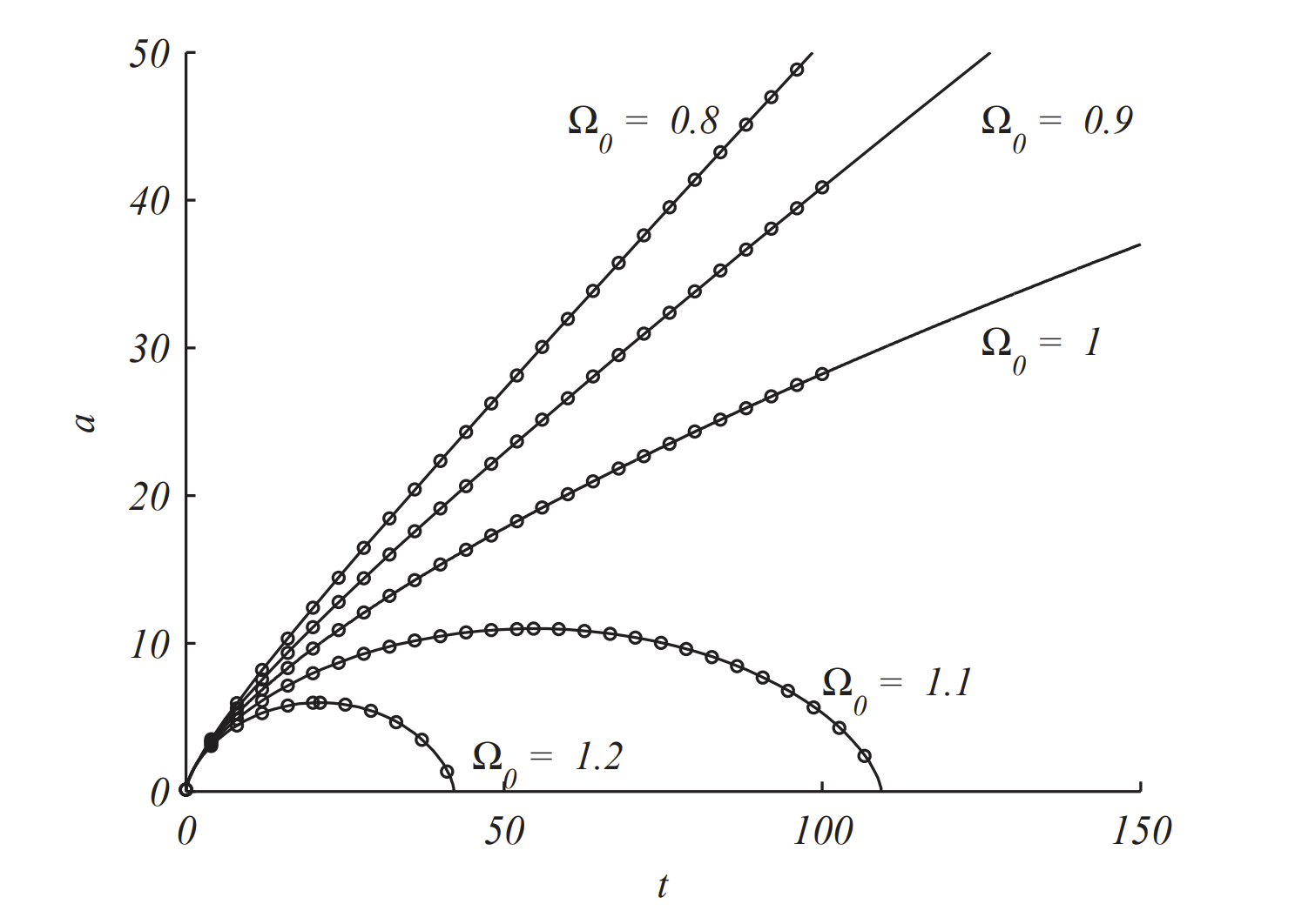
In Figure \(\PageIndex{1}\) we show the results. For \(\Omega_{0}>1\) the solutions lie on the first half of the cycloid solution. The other solutions indicate that the universe continues to expand, leading to what is called the Big Chill. The analytic solutions to the \(\Omega_{0}>1\) cases eventually collapse to \(a=0\) in finite time. These final states are what Stephen Hawking calls the Big Crunch.
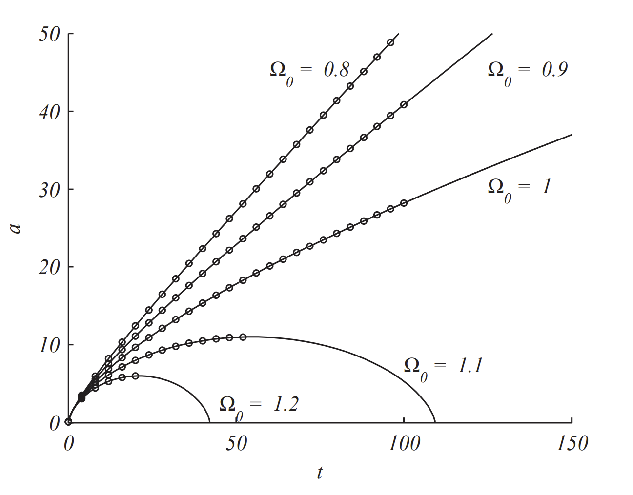
The numerical solutions for \(\Omega_{0}>1\) run into difficulty because the radicand in the square root is negative. But, this corresponds to when \(\dot{a}<0 .\) So, we have to modify the code by estimating the maximum on the curve and run the numerical algorithm with new initial conditions and using the fact that \(\dot{a}<0\) in the function cosmosf by setting da \(=-\operatorname{sqrt}(\mathrm{f})\). The modified code is below and the resulting numerical solutions are shown in Figure \(\PageIndex{2}\).
tspan=0:4:tmax;
a0=.1;
[t,a]=ode45(@cosmosf,tspan,a0);
plot(t,a,’ok’,’MarkerSize’,2)
hold on
if Omega>1
tspan=tmax+.0001:4:2*tmax;
a0=amax-.0001;
[t2,a2]=ode45(@cosmosf2,tspan,a0);
plot(t2,a2,’ok’,’MarkerSize’,2)
end