8.1: Linearization, Critical Points, and Equilibria
- Page ID
- 3414
\( \newcommand{\vecs}[1]{\overset { \scriptstyle \rightharpoonup} {\mathbf{#1}} } \)
\( \newcommand{\vecd}[1]{\overset{-\!-\!\rightharpoonup}{\vphantom{a}\smash {#1}}} \)
\( \newcommand{\id}{\mathrm{id}}\) \( \newcommand{\Span}{\mathrm{span}}\)
( \newcommand{\kernel}{\mathrm{null}\,}\) \( \newcommand{\range}{\mathrm{range}\,}\)
\( \newcommand{\RealPart}{\mathrm{Re}}\) \( \newcommand{\ImaginaryPart}{\mathrm{Im}}\)
\( \newcommand{\Argument}{\mathrm{Arg}}\) \( \newcommand{\norm}[1]{\| #1 \|}\)
\( \newcommand{\inner}[2]{\langle #1, #2 \rangle}\)
\( \newcommand{\Span}{\mathrm{span}}\)
\( \newcommand{\id}{\mathrm{id}}\)
\( \newcommand{\Span}{\mathrm{span}}\)
\( \newcommand{\kernel}{\mathrm{null}\,}\)
\( \newcommand{\range}{\mathrm{range}\,}\)
\( \newcommand{\RealPart}{\mathrm{Re}}\)
\( \newcommand{\ImaginaryPart}{\mathrm{Im}}\)
\( \newcommand{\Argument}{\mathrm{Arg}}\)
\( \newcommand{\norm}[1]{\| #1 \|}\)
\( \newcommand{\inner}[2]{\langle #1, #2 \rangle}\)
\( \newcommand{\Span}{\mathrm{span}}\) \( \newcommand{\AA}{\unicode[.8,0]{x212B}}\)
\( \newcommand{\vectorA}[1]{\vec{#1}} % arrow\)
\( \newcommand{\vectorAt}[1]{\vec{\text{#1}}} % arrow\)
\( \newcommand{\vectorB}[1]{\overset { \scriptstyle \rightharpoonup} {\mathbf{#1}} } \)
\( \newcommand{\vectorC}[1]{\textbf{#1}} \)
\( \newcommand{\vectorD}[1]{\overrightarrow{#1}} \)
\( \newcommand{\vectorDt}[1]{\overrightarrow{\text{#1}}} \)
\( \newcommand{\vectE}[1]{\overset{-\!-\!\rightharpoonup}{\vphantom{a}\smash{\mathbf {#1}}}} \)
\( \newcommand{\vecs}[1]{\overset { \scriptstyle \rightharpoonup} {\mathbf{#1}} } \)
\( \newcommand{\vecd}[1]{\overset{-\!-\!\rightharpoonup}{\vphantom{a}\smash {#1}}} \)
\(\newcommand{\avec}{\mathbf a}\) \(\newcommand{\bvec}{\mathbf b}\) \(\newcommand{\cvec}{\mathbf c}\) \(\newcommand{\dvec}{\mathbf d}\) \(\newcommand{\dtil}{\widetilde{\mathbf d}}\) \(\newcommand{\evec}{\mathbf e}\) \(\newcommand{\fvec}{\mathbf f}\) \(\newcommand{\nvec}{\mathbf n}\) \(\newcommand{\pvec}{\mathbf p}\) \(\newcommand{\qvec}{\mathbf q}\) \(\newcommand{\svec}{\mathbf s}\) \(\newcommand{\tvec}{\mathbf t}\) \(\newcommand{\uvec}{\mathbf u}\) \(\newcommand{\vvec}{\mathbf v}\) \(\newcommand{\wvec}{\mathbf w}\) \(\newcommand{\xvec}{\mathbf x}\) \(\newcommand{\yvec}{\mathbf y}\) \(\newcommand{\zvec}{\mathbf z}\) \(\newcommand{\rvec}{\mathbf r}\) \(\newcommand{\mvec}{\mathbf m}\) \(\newcommand{\zerovec}{\mathbf 0}\) \(\newcommand{\onevec}{\mathbf 1}\) \(\newcommand{\real}{\mathbb R}\) \(\newcommand{\twovec}[2]{\left[\begin{array}{r}#1 \\ #2 \end{array}\right]}\) \(\newcommand{\ctwovec}[2]{\left[\begin{array}{c}#1 \\ #2 \end{array}\right]}\) \(\newcommand{\threevec}[3]{\left[\begin{array}{r}#1 \\ #2 \\ #3 \end{array}\right]}\) \(\newcommand{\cthreevec}[3]{\left[\begin{array}{c}#1 \\ #2 \\ #3 \end{array}\right]}\) \(\newcommand{\fourvec}[4]{\left[\begin{array}{r}#1 \\ #2 \\ #3 \\ #4 \end{array}\right]}\) \(\newcommand{\cfourvec}[4]{\left[\begin{array}{c}#1 \\ #2 \\ #3 \\ #4 \end{array}\right]}\) \(\newcommand{\fivevec}[5]{\left[\begin{array}{r}#1 \\ #2 \\ #3 \\ #4 \\ #5 \\ \end{array}\right]}\) \(\newcommand{\cfivevec}[5]{\left[\begin{array}{c}#1 \\ #2 \\ #3 \\ #4 \\ #5 \\ \end{array}\right]}\) \(\newcommand{\mattwo}[4]{\left[\begin{array}{rr}#1 \amp #2 \\ #3 \amp #4 \\ \end{array}\right]}\) \(\newcommand{\laspan}[1]{\text{Span}\{#1\}}\) \(\newcommand{\bcal}{\cal B}\) \(\newcommand{\ccal}{\cal C}\) \(\newcommand{\scal}{\cal S}\) \(\newcommand{\wcal}{\cal W}\) \(\newcommand{\ecal}{\cal E}\) \(\newcommand{\coords}[2]{\left\{#1\right\}_{#2}}\) \(\newcommand{\gray}[1]{\color{gray}{#1}}\) \(\newcommand{\lgray}[1]{\color{lightgray}{#1}}\) \(\newcommand{\rank}{\operatorname{rank}}\) \(\newcommand{\row}{\text{Row}}\) \(\newcommand{\col}{\text{Col}}\) \(\renewcommand{\row}{\text{Row}}\) \(\newcommand{\nul}{\text{Nul}}\) \(\newcommand{\var}{\text{Var}}\) \(\newcommand{\corr}{\text{corr}}\) \(\newcommand{\len}[1]{\left|#1\right|}\) \(\newcommand{\bbar}{\overline{\bvec}}\) \(\newcommand{\bhat}{\widehat{\bvec}}\) \(\newcommand{\bperp}{\bvec^\perp}\) \(\newcommand{\xhat}{\widehat{\xvec}}\) \(\newcommand{\vhat}{\widehat{\vvec}}\) \(\newcommand{\uhat}{\widehat{\uvec}}\) \(\newcommand{\what}{\widehat{\wvec}}\) \(\newcommand{\Sighat}{\widehat{\Sigma}}\) \(\newcommand{\lt}{<}\) \(\newcommand{\gt}{>}\) \(\newcommand{\amp}{&}\) \(\definecolor{fillinmathshade}{gray}{0.9}\)Except for a few brief detours in Chapter 1, we considered mostly linear equations. Linear equations suffice in many applications, but in reality most phenomena require nonlinear equations. Nonlinear equations, however, are notoriously more difficult to understand than linear ones, and many strange new phenomena appear when we allow our equations to be nonlinear.
Not to worry, we did not waste all this time studying linear equations. Nonlinear equations can often be approximated by linear ones if we only need a solution "locally," for example, only for a short period of time, or only for certain parameters. Understanding linear equations can also give us qualitative understanding about a more general nonlinear problem. The idea is similar to what you did in calculus in trying to approximate a function by a line with the right slope.
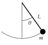
In Section 2.4 we looked at the pendulum of mass \(m\) and length \(L\). The goal was to solve for the angle \(\theta(t)\) as a function of the time \(t\). The equation for the setup is the nonlinear equation
\[\theta'' + \frac{g}{L} \sin \theta = 0 . \nonumber \]

Instead of solving this equation, we solved the rather easier linear equation
\[\theta'' + \frac{g}{L} \theta = 0 . \nonumber \]
While the solution to the linear equation is not exactly what we were looking for, it is rather close to the original, as long as the angle \(\theta\) is small and the time period involved is short.
You might ask: Why don't we just solve the nonlinear problem? Well, it might be very difficult, impractical, or impossible to solve analytically,depending on the equation in question. We may not even be interested in the actual solution, we might only be interested in some qualitative idea of what the solution is doing. For example, what happens as time goes to infinity?
Autonomous Systems and Phase Plane Analysis
We restrict our attention to a two dimensional autonomous system
\[x' = f(x,y) , \qquad y' = g(x,y) , \nonumber \]
where \(f(x,y)\) and \(g(x,y)\) are functions of two variables, and the derivatives are taken with respect to time \(t\). Solutions are functions \(x(t)\) and \(y(t)\) such that
\[x'(t) = f\bigl(x(t),y(t)\bigr), \qquad y'(t) = g\bigl(x(t),y(t)\bigr) . \nonumber \]
The way we will analyze the system is very similar to Section 1.6, where we studied a single autonomous equation. The ideas in two dimensions are the same, but the behavior can be far more complicated.
It may be best to think of the system of equations as the single vector equation
\[\label{eq:1}\begin{bmatrix} x \\ y \end{bmatrix} ' = \begin{bmatrix} f(x,y) \\ g(x,y) \end{bmatrix} . \]
As in Section 3.1 we draw the phase portrait (or phase diagram), where each point \((x,y)\) corresponds to a specific state of the system. We draw the vector field given at each point \((x,y)\) by the vector \(\left[ \begin{smallmatrix} f(x,y) \\ g(x,y) \end{smallmatrix} \right]\). And as before if we find solutions, we draw the trajectories by plotting all points \(\bigl(x(t),y(t)\bigr)\) for a certain range of \(t\).
Consider the second order equation \(x''=-x+x^2\). Write this equation as a first order nonlinear system
\[x' = y , \qquad y' = -x+x^2 . \nonumber \]
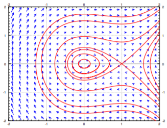
The phase portrait with some trajectories is drawn in Figure \(\PageIndex{2}\).

From the phase portrait it should be clear that even this simple system has fairly complicated behavior. Some trajectories keep oscillating around the origin, and some go off towards infinity. We will return to this example often, and analyze it completely in this (and the next) section.
If we zoom into the diagram near a point where \(\left[ \begin{smallmatrix} f(x,y) \\ g(x,y) \end{smallmatrix} \right]\) is not zero, then nearby the arrows point generally in essentially that same direction and have essentially the same magnitude. In other words the behavior is not that interesting near such a point. We are of course assuming that \(f(x,y)\) and \(g(x,y)\) are continuous.
Let us concentrate on those points in the phase diagram above where the trajectories seem to start, end, or go around. We see two such points: \((0,0)\) and \((1,0)\). The trajectories seem to go around the point \((0,0)\), and they seem to either go in or out of the point \((1,0)\). These points are precisely those points where the derivatives of both \(x\) and \(y\) are zero. Let us define the critical points as the points \((x,y)\) such that
\[ \begin{bmatrix} f(x,y) \\ g(x,y) \end{bmatrix} = \vec{0} . \nonumber \]
In other words, the points where both \(f(x,y)=0\) and \(g(x,y)=0\).
The critical points are where the behavior of the system is in some sense the most complicated. If \(\left[ \begin{smallmatrix} f(x,y) \\ g(x,y) \end{smallmatrix} \right]\) is zero, then nearby, the vector can point in any direction whatsoever. Also, the trajectories are either going towards, away from, or around these points, so if we are looking for long term behavior of the system, we should look at what happens there.
Critical points are also sometimes called equilibria, since we have so-called equilibrium solutions at critical points. If \((x_0,y_0)\) is a critical point, then we have the solutions
\[x(t) = x_0, \quad y(t) = y_0 . \nonumber \]
In Example \(\PageIndex{1}\), there are two equilibrium solutions:
\[x(t) = 0, \quad y(t) = 0, \qquad \text{and} \qquad x(t) = 1, \quad y(t) = 0. \nonumber \]
Compare this discussion on equilibria to the discussion in Section 1.6. The underlying concept is exactly the same.
Linearization
In Section 3.5 we studied the behavior of a homogeneous linear system of two equations near a critical point. For a linear system of two variables the only critical point is generally the origin \((0,0)\). Let us put the understanding we gained in that section to good use understanding what happens near critical points of nonlinear systems.
In calculus we learned to estimate a function by taking its derivative and linearizing. We work similarly with nonlinear systems of ODE. Suppose \((x_0,y_0)\) is a critical point. First change variables to \((u,v)\), so that \((u,v)=(0,0)\) corresponds to \((x_0,y_0)\). That is,
\[u=x-x_0, \qquad v=y-y_0 . \nonumber \]
Next we need to find the derivative. In multivariable calculus you may have seen that the several variables version of the derivative is the Jacobian matrix\(^{1}\). The Jacobian matrix of the vector-valued function \(\left[ \begin{smallmatrix} f(x,y) \\ g(x,y) \end{smallmatrix} \right]\) at \((x_0,y_0)\) is
\[ \begin{bmatrix}\frac{\partial f}{\partial x}(x_0,y_0) ~~~~ \frac{\partial f}{\partial y}(x_0,y_0) \\ \frac{\partial g}{\partial x}(x_0,y_0) ~~~~ \frac{\partial g}{\partial y}(x_0,y_0) \end{bmatrix} . \nonumber \]
This matrix gives the best linear approximation as \(u\) and \(v\) (and therefore \(x\) and \(y\)) vary. We define the linearization of the equation \(\eqref{eq:1}\) as the linear system
\[ \begin{bmatrix} u \\ v \end{bmatrix} ' = \begin{bmatrix} \frac{\partial f}{\partial x}(x_0,y_0) ~~~ ~\frac{\partial f}{\partial y}(x_0,y_0) \\ \frac{\partial g}{\partial x}(x_0,y_0)~~~~ \frac{\partial g}{\partial y}(x_0,y_0) \end{bmatrix} \begin{bmatrix} u \\ v \end{bmatrix} . \nonumber \]
Let us keep with the same equations as Example \(\PageIndex{1}\): \(x' = y\), \(y' = -x+x^2\). There are two critical points, \((0,0)\)and \((1,0)\). The Jacobian matrix at any point is
\[\begin{bmatrix} \frac{\partial f}{\partial x}(x,y) ~~~~ \frac{\partial f}{\partial y}(x,y) \\ \frac{\partial g}{\partial x}(x,y) ~~~~ \frac{\partial g}{\partial y}(x,y) \end{bmatrix} = \begin{bmatrix} 0 & 1 \\ -1+2x & 0 \end{bmatrix}. \nonumber \]
Therefore at \((0,0)\), we have \(u=x\) and \(v=y\), and the linearization is
\[\begin{bmatrix} u \\ v \end{bmatrix} ' =\begin{bmatrix}0 & 1 \\-1 & 0\end{bmatrix}\begin{bmatrix} u \\ v \end{bmatrix} , \nonumber \]
where \(u=x\) and \(v=y\).
At the point \((1,0)\), we have \(u=x-1\) and \(v=y\), and the linearization is
\[\begin{bmatrix} u \\ v \end{bmatrix} ' =\begin{bmatrix}0 & 1 \\1 & 0\end{bmatrix}\begin{bmatrix} u \\ v \end{bmatrix} . \nonumber \]
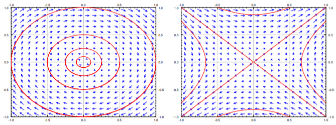
The phase diagrams of the two linearizations at the point \((0,0)\) and \((1,0)\) are given in Figure \(\PageIndex{3}\). Note that the variables are now \(u\) and \(v\). Compare Figure \(\PageIndex{3}\) with Figure \(\PageIndex{2}\), and look especially at the behavior near the critical points.

Footnotes
[1] Named for the German mathematician Carl Gustav Jacob Jacobi (1804–1851).


