2.1: Introduction

In this chapter we will introduce several generic second order linear partial differential equations and see how such equations lead naturally to the study of boundary value problems for ordinary differential equations. These generic differential equation occur in one to three spatial dimensions and are all linear differential equations. A list is provided in Table \(\PageIndex{1}\). Here we have introduced the Laplacian operator, \(∇^2u = u_{xx} + u_{yy} + u_{zz}\). Depending on the types of boundary conditions imposed and on the geometry of the system (rectangular, cylindrical, spherical, etc.), one encounters many interesting boundary value problems.

Table \(\PageIndex{1}\): List of generic partial differential equations.

Name	2 Vars	3D
Heat Equation	\(u_t=ku_{xx}\)	\(u_t=k\nabla ^2u\)
Wave Equation	\(u_{tt}=c^2u_{xx}\)	\(u_{tt}=c^2\nabla^2u\)
Laplace's Equation	\(u_{xx}+u_{yy}=0\)	\(\nabla^2u=0\)
Poisson's Equation	\(u_{xx}+u_{yy}=F(x,y)\)	\(\nabla^2u=F(x,y,z)\)
Schrödinger’s Equation	\(iu_t=u_{xx}+F(x,t)u\)	\(iu_t=\nabla^2u+F(x,y,z,t)u\)

Let’s look at the heat equation in one dimension. This could describe the heat conduction in a thin insulated rod of length \(L\). It could also describe the diffusion of pollutant in a long narrow stream, or the flow of traffic down a road. In problems involving diffusion processes, one instead calls this equation the diffusion equation. [See the derivation in Section 2.2.2.]

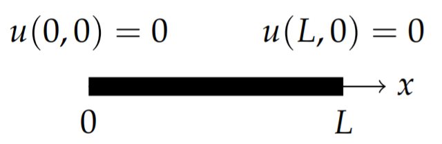
A typical initial-boundary value problem for the heat equation would be that initially one has a temperature distribution \(u(x, 0) = f(x)\). Placing the bar in an ice bath and assuming the heat flow is only through the ends of the bar, one has the boundary conditions \(u(0, t) = 0\) and \(u(L, t) = 0\). Of course, we are dealing with Celsius temperatures and we assume there is plenty of ice to keep that temperature fixed at each end for all time as seen in Figure \(\PageIndex{1}\). So, the problem one would need to solve is given as [IC = initial condition(s) and BC = boundary conditions.]

Figure \(\PageIndex{1}\): One dimensional heated rod of length \(L\).

Heat Equation

\[\begin{array}{lcc} \text{PDE}& u_t=ku_{xx}, &0<t,\quad 0\leq x\leq L, \\ \text{IC}& u(x,0)=f(x), & 0<<L, \\ \text{BC}&u(0,t)=0,&t>0, \\ &u(L,t)=0,&t>0,\end{array}\label{eq:1}\] Here, \(k\) is the heat conduction constant and is determined using properties of the bar.

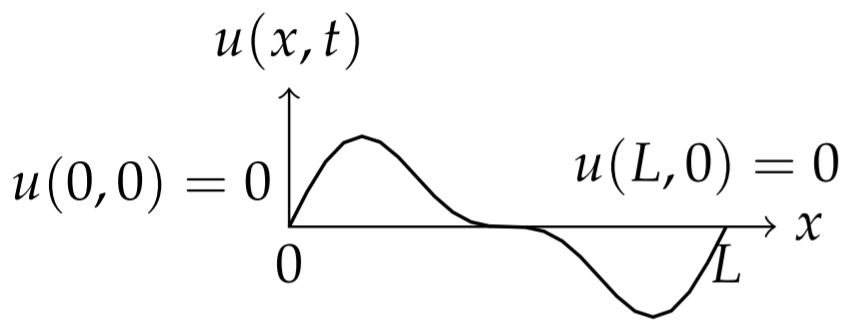
Another problem that will come up in later discussions is that of the vibrating string. A string of length \(L\) is stretched out horizontally with both ends fixed such as a violin string as shown in Figure \(\PageIndex{2}\). Let \(u(x, t)\) be the vertical displacement of the string at position \(x\) and time \(t\). The motion of the string is governed by the one dimensional wave equation. [See the derivation in Section 2.2.1.] The string might be plucked, giving the string an initial profile, \(u(x, 0) = f(x)\), and possibly each point on the string has an initial velocity \(u_t(x, 0) = g(x)\). The initial-boundary value problem for this problem is given below.

Wave Equation

\[\begin{array}{lcc}\text{PDE}&u_{tt}=c^2u_{xx}&0<t,\quad 0\leq x\leq L \\ \text{IC}&u(x,0)=f(x)&0<x<L \\ &u_t(x,0)=g(x)&0<x<L \\ \text{BC}&u(0,t)=0&t>0 \\ &u(L,t)=0&t>0\end{array}\label{eq:2}\] In this problem \(c\) is the wave speed in the string. It depends on the mass per unit length of the string, \(\mu\), and the tension, \(τ\), placed on the string.

Figure \(\PageIndex{2}\): One dimensional string of length \(L\).

There is a rich history on the study of these and other partial differential equations and much of this involves trying to solve problems in physics. Consider the one dimensional wave motion in the string. Physically, the speed of these waves depends on the tension in the string and its mass density. The frequencies we hear are then related to the string shape, or the allowed wavelengths across the string. We will be interested the harmonics, or pure sinusoidal waves, of the vibrating string and how a general wave on the string can be represented as a sum over such harmonics. This will take us into the field of spectral, or Fourier, analysis. The solution of the heat equation also involves the use of Fourier analysis. However, in this case there are no oscillations in time.

There are many applications that are studied using spectral analysis. At the root of these studies is the belief that continuous waveforms are comprised of a number of harmonics. Such ideas stretch back to the Pythagoreans study of the vibrations of strings, which led to their program of a world of harmony. This idea was carried further by Johannes Kepler (1571-1630) in his harmony of the spheres approach to planetary orbits. In the 1700’s others worked on the superposition theory for vibrating waves on a stretched spring, starting with the wave equation and leading to the superposition of right and left traveling waves. This work was carried out by people such as John Wallis (1616-1703), Brook Taylor (1685-1731) and Jean le Rond d’Alembert (1717-1783).

Figure \(\PageIndex{3}\): Plot of the second harmonic of a vibrating string at different times.

In 1742 d’Alembert solved the wave equation

\[c^2\frac{\partial ^2y}{\partial x^2}-\frac{\partial ^2y}{\partial t^2}=0,\nonumber\]

where \(y\) is the string height and \(c\) is the wave speed. However, this solution led him and others, like Leonhard Euler (1707-1783) and Daniel Bernoulli (1700-1782), to investigate what "functions" could be the solutions of this equation. In fact, this led to a more rigorous approach to the study of analysis by first coming to grips with the concept of a function. For example, in 1749 Euler sought the solution for a plucked string in which case the initial condition \(y(x, 0) = h(x)\) has a discontinuous derivative! (We will see how this led to important questions in analysis.)

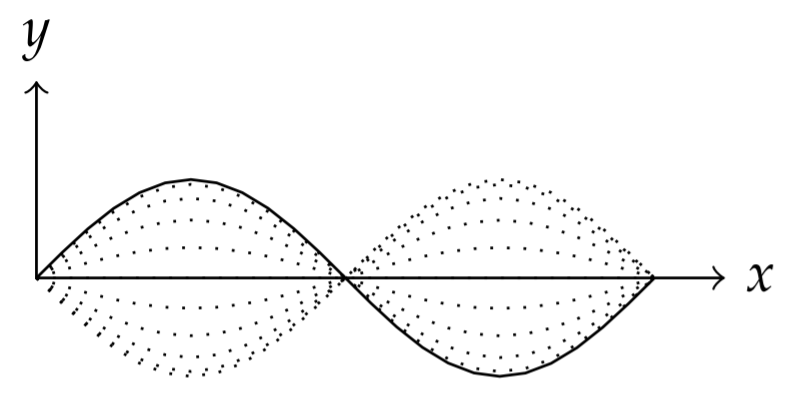
In 1753 Daniel Bernoulli viewed the solutions as a superposition of simple vibrations, or harmonics. Such superpositions amounted to looking at solutions of the form

\[y(x,t)=\sum\limits_k a_k\sin\frac{k\pi x}{L}\cos\frac{k\pi ct}{L},\nonumber\]

where the string extends over the interval \([0, L]\) with fixed ends at \(x = 0\) and \(x = L\).

However, the initial profile for such superpositions is given by

\[y(x,0)=\sum\limits_k a_k\sin\frac{k\pi x}{L}.\nonumber\]

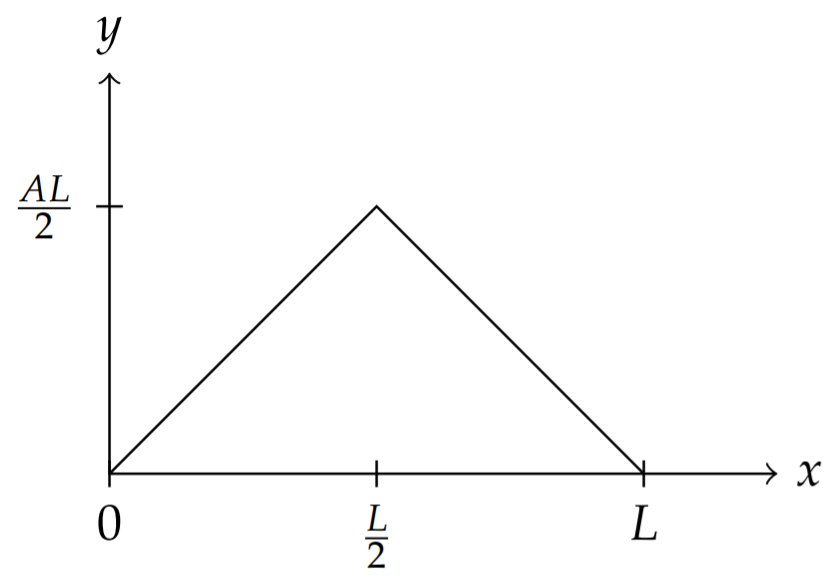
It was determined that many functions could not be represented by a finite number of harmonics, even for the simply plucked string in Figure \(\PageIndex{4}\) given by an initial condition of the form

\[y(x,0)=\left\{\begin{array}{cc}Ax, &0\leq x\leq L/2 \\ A(L-x),&L/2\leq x\leq L\end{array}\right.\nonumber\]

Thus, the solution consists generally of an infinite series of trigonometric functions.

Figure \(\PageIndex{4}\): Plot of an initial condition for a plucked string.

Note

The one dimensional version of the heat equation is a partial differential equation for \(u(x, t)\) of the form \[\frac{\partial u}{\partial t}=k\frac{\partial ^2u}{\partial x^2}.\nonumber\]

Solutions satisfying boundary conditions \(u(0, t) = 0\) and \(u(L, t) = 0\), are of the form \[u(x,t)=\sum\limits_{n=0}^\infty b_n\sin\frac{n\pi x}{L}e^{-n^2\pi^2 t/L^2}.\nonumber\]

In this case, setting \(u(x, 0) = f(x)\), one has to satisfy the condition \[f(x)=\sum\limits_{n=0}^\infty b_n\sin\frac{n\pi x}{L}.\nonumber\] This is another example leading to an infinite series of trigonometric functions.

Such series expansions were also of importance in Joseph Fourier’s (1768- 1830) solution of the heat equation. The use of Fourier expansions has become an important tool in the solution of linear partial differential equations, such as the wave equation and the heat equation. More generally, using a technique called the Method of Separation of Variables, allowed higher dimensional problems to be reduced to one dimensional boundary value problems. However, these studies led to very important questions, which in turn opened the doors to whole fields of analysis. Some of the problems raised were

1. What functions can be represented as the sum of trigonometric functions?
2. How can a function with discontinuous derivatives be represented by a sum of smooth functions, such as the above sums of trigonometric functions?
3. Do such infinite sums of trigonometric functions actually converge to the functions they represent?

There are many other systems for which it makes sense to interpret the solutions as sums of sinusoids of particular frequencies. For example, we can consider ocean waves. Ocean waves are affected by the gravitational pull of the moon and the sun and other numerous forces. These lead to the tides, which in turn have their own periods of motion. In an analysis of wave heights, one can separate out the tidal components by making use of Fourier analysis.

In the Section 2.4 we describe how to go about solving these equations using the method of separation of variables. We will find that in order to accommodate the initial conditions, we will need to introduce Fourier series before we can complete the problems, which will be the subject of the following chapter. However, we first derive the one-dimensional wave and heat equations.