
2.2: Derivation of Generic 1D Equations


- Last updated
- Sep 4, 2024
- Save as PDF

( \newcommand{\kernel}{\mathrm{null}\,}\)
Derivation of Wave Equation for String
The wave equation for a one dimensional string is derived based upon simply looking at Newton’s Second Law of Motion for a piece of the string plus a few simple assumptions, such as small amplitude oscillations and constant density.
We begin with F=ma. The mass of a piece of string of length ds is m=ρ(x)ds. From Figure 2.2.1 an incremental length f the string is given by
Δs2=Δx2+Δu2.
The piece of string undergoes an acceleration of a=∂2u∂t2.
We will assume that the main force acting on the string is that of tension. Let T(x,t) be the magnitude of the tension acting on the left end of the piece of string. Then, on the right end the tension is T(x + ∆x, t). At these points the tension makes an angle to the horizontal of θ(x, t) and θ(x + ∆x, t), respectively.
Assuming that there is no horizontal acceleration, the x-component in the second law, m\mathbf{a} = \mathbf{F}, for the string element is given by
0=T(x+\Delta x,t)\cos\theta (x+\Delta x,t)-T(x,t)\cos\theta (x,t).\nonumber

The vertical component is given by
\rho (x)\Delta s\frac{\partial ^2u}{\partial t^2}=T(x+\Delta x,t)\sin\theta (x+\Delta x,t)-T(x,t)\sin\theta(x,t)\nonumber
The length of the piece of string can be written in terms of ∆x,
\Delta s=\sqrt{\Delta x^2+\Delta u^2}=\sqrt{1+\left(\frac{\Delta u}{\Delta x}\right)^2}\Delta x.\nonumber
and the right hand sides of the component equation can be expanded about ∆x = 0, to obtain
\begin{aligned}T(x+\Delta x,t)\cos\theta (x+\Delta x,t)-T(x,t)\cos\theta (x,t)&\approx\frac{\partial (T\cos\theta)}{\partial x}(x,t)\Delta x \\ T(x+\Delta x,t)\sin\theta (x+\Delta x,t)-T(x,t)\sin\theta (x,t)&\approx\frac{\partial (T\sin\theta )}{\partial x}(x,t)\Delta x.\end{aligned} \nonumber
Furthermore, we note that
\tan\theta =\lim\limits_{\Delta x\to 0}\frac{\Delta u}{\Delta x}=\frac{\partial u}{\partial x}.\nonumber
Now we can divide these component equations by ∆x and let ∆x → 0. This gives the approximations
\begin{align}0&=\frac{T(x+\Delta x,t)\cos\theta (x+\Delta x,t)-T(x,t)\cos\theta (x,t)}{\Delta x}\nonumber \\ &\approx\frac{\partial (T\cos\theta)}{\partial x}(x,t)\nonumber \\ \rho(x)\frac{\partial^2u}{\partial t^2}\frac{\delta s}{\delta s}&=\frac{T(x+\Delta x,t)\sin\theta (x+\Delta x,t)-T(x,t)\sin\theta (x,t)}{\Delta x}\nonumber \\ \rho (x)\frac{\partial ^2u}{\partial t^2}\sqrt{1+\left(\frac{\partial u}{\partial x}\right)^2}&\approx \frac{\partial (T\sin\theta)}{\partial x}(x,t).\label{eq:1}\end{align}
We will assume a small angle approximation, giving
\sin\theta\approx\tan\theta =\frac{\partial u}{\partial x},\nonumber
\cos\theta\approx 1, and
\sqrt{1+\left(\frac{\partial u}{\partial x}\right)^2}\approx 1.\nonumber
Then, the horizontal component becomes
\frac{\partial T(x,t)}{\partial x}=0.\nonumber
Therefore, the magnitude of the tension T(x, t) = T(t) is at most time dependent.
The vertical component equation is now
\rho (x)\frac{\partial ^2u}{\partial t^2}=T(t)\frac{\partial}{\partial x}\left(\frac{\partial u}{\partial x}\right)=T(t)\frac{\partial ^2u}{\partial x^2}.\nonumber
Assuming that ρ and T are constant and defining
c^2=\frac{T}{\rho},\nonumber
we obtain the one dimensional wave equation,
\frac{\partial ^2u}{\partial t^2}=c^2\frac{\partial ^2u}{\partial x^2}.\nonumber
Derivation of 1D Heat Equation
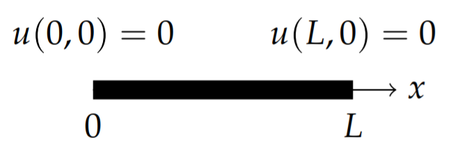
Consider a one dimensional rod of length L as shown in Figure \PageIndex{2}. It is heated and allowed to sit. The heat equation is the governing equation which allows us to determine the temperature of the rod at a later time.
We begin with some simple thermodynamics. Recall that to raise the temperature of a mass m by ∆T takes thermal energy given by
Q=mc\Delta T,\nonumber
assuming the mass does not go through a phase transition. Here c is the specific heat capacity of the substance. So, we will begin with the heat content of the rod as
Q=mcT(x,t)\nonumber
and assume that m and c are constant.
We will also need Fourier’s law of heat transfer or heat conduction. This law simply states that heat energy flows from warmer to cooler regions and is written in terms of the heat energy flux, \phi (x, t). The heat energy flux, or flux density, gives the rate of energy flow per area. Thus, the amount of heat energy flowing over the left end of the region of cross section A in time ∆t is given \phi (x, t)∆tA. The units of \phi (x, t) are then \text{J/s/m}^2 = \text{W/m}^2.
Fourier’s law of heat conduction states that the flux density is proportional to the gradient of the temperature,
\phi =-K\frac{\partial T}{\partial x}.\nonumber
Here K is the thermal conductivity and the negative sign takes into account the direction of flow from higher to lower temperatures.
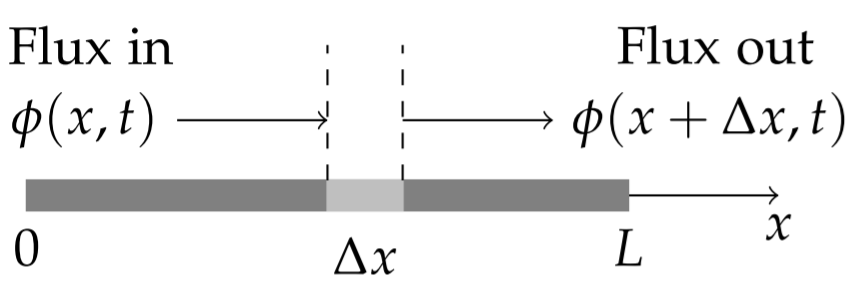
Now we make use of the conservation of energy. Consider a small section of the rod of width ∆x as shown in Figure \PageIndex{3}. The rate of change of the energy through this section is due to energy flow through the ends. Namely
\text{Rate of change of heat energy }=\text{ Heat in }-\text{ Heat out}.\nonumber
The energy content of the small segment of the rod is given by
\Delta Q=(ρA∆x)cT(x, t + ∆t) − (ρA∆x)cT(x, t).\nonumber
The flow rates across the boundaries are given by the flux.
(ρA∆x)cT(x, t + ∆t) − (ρA∆x)cT(x, t) = [\phi (x, t) − \phi (x + ∆x, t)]∆tA.\nonumber
Dividing by ∆x and ∆t and letting ∆x, ∆t → 0, we obtain
\frac{\partial T}{\partial t}=-\frac{1}{c\rho}\frac{\partial\phi}{\partial x}.\nonumber
Using Fourier’s law of heat conduction,
\frac{\partial T}{\partial t}=\frac{1}{c\rho}\frac{\partial}{\partial x}\left(K\frac{\partial T}{\partial x}\right).\nonumber
Assuming K, c, and ρ are constant, we have the one dimensional heat equation as used in the text:
\frac{\partial T}{\partial t}=k\frac{\partial ^2T}{\partial x^2},\nonumber
where k=\frac{k}{c\rho}.