4.2: Properties of Sturm-Liouville Eigenvalue Problems

There are several properties that can be proven for the (regular) Sturm-Liouville eigenvalue problem in (4.1.3). However, we will not prove them all here. We will merely list some of the important facts and focus on a few of the properties.

1. The eigenvalues are real, countable, ordered and there is a smallest eigenvalue. Thus, we can write them as \(\lambda_{1}<\lambda_{2}<\ldots\). However, there is no largest eigenvalue and \(n \rightarrow \infty, \lambda_{n} \rightarrow \infty\).
2. For each eigenvalue \(\lambda_{n}\) there exists an eigenfunction \(\phi_{n}\) with \(n-1\) zeros on \((a, b)\).
3. Eigenfunctions corresponding to different eigenvalues are orthogonal with respect to the weight function, \(\sigma(x)\). Defining the inner product of \(f(x)\) and \(g(x)\) as \[\langle f, g\rangle=\int_{a}^{b} f(x) g(x) \sigma(x) d x,\label{eq:1}\] then the orthogonality of the eigenfunctions can be written in the form \[\left\langle\phi_{n}, \phi_{m}\right\rangle=\left\langle\phi_{n}, \phi_{n}\right\rangle \delta_{n m}, \quad n, m=1,2, \ldots .\label{eq:2}\]
4. The set of eigenfunctions is complete; i.e., any piecewise smooth function can be represented by a generalized Fourier series expansion of the eigenfunctions, \[f(x) \sim \sum_{n=1}^{\infty} c_{n} \phi_{n}(x),\nonumber \] where \[c_{n}=\frac{\left\langle f, \phi_{n}\right\rangle}{\left\langle\phi_{n}, \phi_{n}\right\rangle} .\nonumber \] Actually, one needs \(f(x) \in L_{\sigma}^{2}(a, b)\), the set of square integrable functions over \([a, b]\) with weight function \(\sigma(x)\). By square integrable, we mean that \(\langle f, f\rangle\langle\infty\). One can show that such a space is isomorphic to a Hilbert space, a complete inner product space. Hilbert spaces play a special role in quantum mechanics.
5. The eigenvalues satisfy the Rayleigh quotient \[\lambda_{n}=\frac{-\left.p \phi_{n} \frac{d \phi_{n}}{d x}\right|_{a} ^{b}+\int_{a}^{b}\left[p\left(\frac{d \phi_{n}}{d x}\right)^{2}-q \phi_{n}^{2}\right] d x}{\left\langle\phi_{n}, \phi_{n}\right\rangle} .\nonumber \] This is verified by multiplying the eigenvalue problem \[\mathcal{L} \phi_{n}=-\lambda_{n} \sigma(x) \phi_{n}\nonumber \] by \(\phi_{n}\) and integrating. Solving this result for \(\lambda_{n}\), we obtain the Rayleigh quotient. The Rayleigh quotient is useful for getting estimates of eigenvalues and proving some of the other properties.

Example \(\PageIndex{1}\)

Verify some of these properties for the eigenvalue problem \[y^{\prime \prime}=-\lambda y, \quad y(0)=y(\pi)=0 .\]

Solution

This is a problem we had seen many times. The eigenfunctions for this eigenvalue problem are \(\phi_{n}(x)=\sin n x\), with eigenvalues \(\lambda_{n}=n^{2}\) for \(n=1,2, \ldots\). These satisfy the properties listed above.

First of all, the eigenvalues are real, countable and ordered, \(1<4<9<\ldots\). There is no largest eigenvalue and there is a first one.

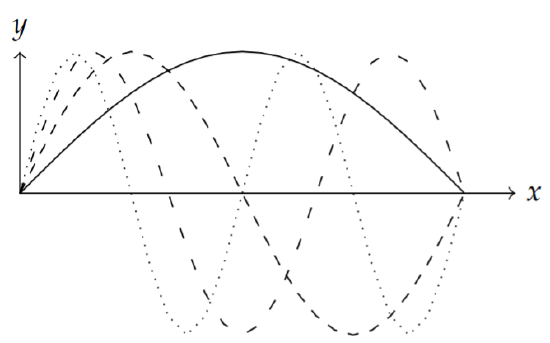
The eigenfunctions corresponding to each eigenvalue have \(n-1\) zeros on \((0, \pi)\). \(\phi_{n}(x)=\sin n x\) for \(n=1,2,3,4\) This is demonstrated for several eigenfunctions in Figure \(\PageIndex{1}\).

Figure \(\PageIndex{1}\): Plot of the eigenfunctions \(\phi_n(x)\sin nx\) for \(n=1,2,3,4\).

We also know that the set \(\{\sin n x\}_{n=1}^{\infty}\) is an orthogonal set of basis functions of length \[||\phi_n|| =\sqrt{\frac{\pi}{2}}.\nonumber\] Thus, the Rayleigh quotient can be computed using \(p(x)=1\), \(q(x)=0\), and the eigenfunctions it is given by \[\begin{aligned} R&=\frac{-\left.\phi_{n} \phi_{n}^{\prime}\right|_{0} ^{\pi}+\int_{0}^{\pi}\left(\phi_{n}^{\prime}\right)^{2} d x}{\frac{\pi}{2}} \\ &=\frac{2}{\pi}\int_0^\pi (-n^2\cos nx)^2dx=n^2. \end{aligned}\]

Therefore, knowing the eigenfunction, the Rayleigh quotient returns the eigenvalues as expected.

Example \(\PageIndex{2}\)

We seek the eigenfunctions of the operator found in Example 4.1.1. Namely, we want to solve the eigenvalue problem \[\mathcal{L} y=\left(x y^{\prime}\right)^{\prime}+\frac{2}{x} y=-\lambda \sigma y\label{eq:4}\] subject to a set of homogeneous boundary conditions. Let’s use the boundary conditions \[y^{\prime}(1)=0, \quad y^{\prime}(2)=0 .\nonumber \] [Note that we do not know \(\sigma(x)\) yet, but will choose an appropriate function to obtain solutions.]

Solution

Expanding the derivative, we have \[x y^{\prime \prime}+y^{\prime}+\frac{2}{x} y=-\lambda \sigma y \text {. }\nonumber \] Multiply through by \(x\) to obtain \[x^{2} y^{\prime \prime}+x y^{\prime}+(2+\lambda x \sigma) y=0 .\nonumber \] Notice that if we choose \(\sigma(x)=x^{-1}\), then this equation can be made a Cauchy-Euler type equation. Thus, we have \[x^{2} y^{\prime \prime}+x y^{\prime}+(\lambda+2) y=0 .\nonumber \] The characteristic equation is \[r^{2}+\lambda+2=0 .\nonumber \] For oscillatory solutions, we need \(\lambda+2>0\). Thus, the general solution is \[y(x)=c_{1} \cos (\sqrt{\lambda+2} \ln |x|)+c_{2} \sin (\sqrt{\lambda+2} \ln |x|) \text {. }\label{eq:5}\]

Next we apply the boundary conditions. \(y^{\prime}(1)=0\) forces \(c_{2}=0\). This leaves \[y(x)=c_{1} \cos (\sqrt{\lambda+2} \ln x) .\nonumber \] The second condition, \(y^{\prime}(2)=0\), yields \[\sin (\sqrt{\lambda+2} \ln 2)=0 .\nonumber \] This will give nontrivial solutions when \[\sqrt{\lambda+2} \ln 2=n \pi, \quad n=0,1,2,3 \ldots .\nonumber \]

In summary, the eigenfunctions for this eigenvalue problem are \[y_{n}(x)=\cos \left(\frac{n \pi}{\ln 2} \ln x\right), \quad 1 \leq x \leq 2\nonumber \] and the eigenvalues are \(\lambda_{n}=\left(\frac{n \pi}{\ln 2}\right)^{2}-2\) for \(n=0,1,2, \ldots\)

Note

We include the \(n=0\) case because \(y(x)=\) constant is a solution of the \(\lambda=-2\) case. More specifically, in this case the characteristic equation reduces to \(r^{2}=0\). Thus, the general solution of this Cauchy-Euler equation is \[y(x)=c_{1}+c_{2} \ln |x| .\nonumber \] Setting \(y^{\prime}(1)=0\), forces \(c_{2}=0 . y^{\prime}(2)\) automatically vanishes, leaving the solution in this case as \(y(x)=c_{1}\).

We note that some of the properties listed in the beginning of the section hold for this example. The eigenvalues are seen to be real, countable and ordered. There is a least one, \(\lambda_{0}=-2\). Next, one can find the zeros of each eigenfunction on \([1,2]\). Then the argument of the cosine, \(\frac{n \pi}{\ln 2} \ln x\), takes values \(0\) to \(n\pi\) for \(x \in[1,2]\). The cosine function has \(n-1\) roots on this interval.

Orthogonality can be checked as well. We set up the integral and use the substitution \(y=\pi \ln x / \ln 2\). This gives \[\begin{align} \left\langle y_{n}, y_{m}\right\rangle &=\int_{1}^{2} \cos \left(\frac{n \pi}{\ln 2} \ln x\right) \cos \left(\frac{m \pi}{\ln 2} \ln x\right) \frac{d x}{x}\nonumber \\ &=\frac{\ln 2}{\pi} \int_{0}^{\pi} \cos n y \cos m y d y\nonumber \\ &=\frac{\ln 2}{2} \delta_{n, m} .\label{eq:6} \end{align}\]

Adjoint Operators

In the study of the spectral theory of matrices, one learns about the adjoint of the matrix, \(A^{\dagger}\), and the role that self-adjoint, or Hermitian, matrices play in diagonalization. Also, one needs the concept of adjoint to discuss the existence of solutions to the matrix problem \(\mathbf{y}=A \mathbf{x}\). In the same spirit, one is interested in the existence of solutions of the operator equation \(L u=f\) and solutions of the corresponding eigenvalue problem. The study of linear operators on a Hilbert space is a generalization of what the reader had seen in a linear algebra course.

Just as one can find a basis of eigenvectors and diagonalize Hermitian, or self-adjoint, matrices (or, real symmetric in the case of real matrices), we will see that the Sturm-Liouville operator is self-adjoint. In this section we will define the domain of an operator and introduce the notion of adjoint operators. In the last section we discuss the role the adjoint plays in the existence of solutions to the operator equation \(L u=f\).

We begin by defining the adjoint of an operator. The adjoint, \(L^{\dagger}\), of operator \(L\) satisfies \[\langle u, L v\rangle=\left\langle L^{+} u, v\right\rangle\nonumber \] for all \(v\) in the domain of \(L\) and \(u\) in the domain of \(L^{+}\). Here the domain of a differential operator \(L\) is the set of all \(u \in L_{\sigma}^{2}(a, b)\) satisfying a given set of homogeneous boundary conditions. This is best understood through example.

Example \(\PageIndex{3}\)

Find the adjoint of \(L=a_{2}(x) D^{2}+a_{1}(x) D+a_{0}(x)\) for \(D=d / d x\).

Solution

In order to find the adjoint, we place the operator inside an integral. Consider the inner product \[\langle u, L v\rangle=\int_{a}^{b} u\left(a_{2} v^{\prime \prime}+a_{1} v^{\prime}+a_{0} v\right) d x .\nonumber \] We have to move the operator \(L\) from \(v\) and determine what operator is acting on \(u\) in order to formally preserve the inner product. For a simple operator like \(L=\frac{d}{d x}\), this is easily done using integration by parts. For the given operator, we will need to apply several integrations by parts to the individual terms. We consider each derivative term in the integrand separately.

For the \(a_{1} v^{\prime}\) term, we integrate by parts to find \[\int_{a}^{b} u(x) a_{1}(x) v^{\prime}(x) d x=\left.a_{1}(x) u(x) v(x)\right|_{a} ^{b}-\int_{a}^{b}\left(u(x) a_{1}(x)\right)^{\prime} v(x) d x .\label{eq:7}\]

Now, we consider the \(a_{2} v^{\prime \prime}\) term. In this case it will take two integrations by parts: \[\begin{align} \int_{a}^{b} u(x) a_{2}(x) v^{\prime \prime}(x) d x=&\left.a_{2}(x) u(x) v^{\prime}(x)\right|_{a} ^{b}-\int_{a}^{b}\left(u(x) a_{2}(x)\right)^{\prime} v(x)^{\prime} d x\nonumber \\ =&\left.\left[a_{2}(x) u(x) v^{\prime}(x)-\left(a_{2}(x) u(x)\right)^{\prime} v(x)\right]\right|_{a} ^{b}\nonumber \\ &+\int_{a}^{b}\left(u(x) a_{2}(x)\right)^{\prime \prime} v(x) d x .\label{eq:8} \end{align}\] Combining these results, we obtain \[\begin{align} \langle u, L v\rangle=& \int_{a}^{b} u\left(a_{2} v^{\prime \prime}+a_{1} v^{\prime}+a_{0} v\right) d x\nonumber \\ =&\left.\left[a_{1}(x) u(x) v(x)+a_{2}(x) u(x) v^{\prime}(x)-\left(a_{2}(x) u(x)\right)^{\prime} v(x)\right]\right|_{a} ^{b}\nonumber \\ &+\int_{a}^{b}\left[\left(a_{2} u\right)^{\prime \prime}-\left(a_{1} u\right)^{\prime}+a_{0} u\right] v d x .\label{eq:9} \end{align}\]

Inserting the boundary conditions for \(v\), one has to determine boundary conditions for \(u\) such that \[\left.\left[a_{1}(x) u(x) v(x)+a_{2}(x) u(x) v^{\prime}(x)-\left(a_{2}(x) u(x)\right)^{\prime} v(x)\right]\right|_{a} ^{b}=0 .\nonumber \] This leaves \[\langle u, L v\rangle=\int_{a}^{b}\left[\left(a_{2} u\right)^{\prime \prime}-\left(a_{1} u\right)^{\prime}+a_{0} u\right] v d x \equiv\left\langle L^{\dagger} u, v\right\rangle .\nonumber \] Therefore, \[L^{\dagger}=\frac{d^{2}}{d x^{2}} a_{2}(x)-\frac{d}{d x} a_{1}(x)+a_{0}(x) .\label{eq:10} \]

When \(L^{\dagger}=L\), the operator is called formally self-adjoint. When the domain of \(L\) is the same as the domain of \(L^{\dagger}\), the term self-adjoint is used. As the domain is important in establishing self-adjointness, we need to do a complete example in which the domain of the adjoint is found.

Example \(\PageIndex{4}\)

Determine \(L^{\dagger}\) and its domain for operator \(L u=\frac{d u}{d x}\) where \(u\) satisfies the boundary conditions \(u(0)=2 u(1)\) on \([0,1]\).

Solution

We need to find the adjoint operator satisfying \(\langle v, L u\rangle=\left\langle L^{\dagger} v, u\right\rangle\). Therefore, we rewrite the integral \[\langle v, L u\rangle\rangle=\int_{0}^{1} v \frac{d u}{d x} d x=\left.u v\right|_{0} ^{1}-\int_{0}^{1} u \frac{d v}{d x} d x=\left\langle L^{+} v, u\right\rangle .\nonumber \] From this we have the adjoint problem consisting of an adjoint operator and the associated boundary condition (or, domain of \(L^{\dagger}\).): \[\begin{aligned} &\text { 1. } L^{\dagger}=-\frac{d}{d x} . \\ &\text { 2. }\left.u v\right|_{0} ^{1}=0 \Rightarrow 0=u(1)[v(1)-2 v(0)] \Rightarrow v(1)=2 v(0) . \end{aligned}\]

Lagrange’s and Green’s Identities

Before turning to the proofs that the eigenvalues of a Sturm-Liouville problem are real and the associated eigenfunctions orthogonal, we will first need to introduce two important identities. For the Sturm-Liouville operator, \[\mathcal{L}=\frac{d}{d x}\left(p \frac{d}{d x}\right)+q,\nonumber \] we have the two identities:

Definition \(\PageIndex{1}\): Lagrange's Identity

\[u \mathcal{L} v-v \mathcal{L} u =\left[p\left(u v^{\prime}-v u^{\prime}\right)\right]^{\prime} .\nonumber\]

Definition \(\PageIndex{2}\): Green's Identity

\[\int_{a}^{b}(u \mathcal{L} v-v \mathcal{L} u) d x =\left.\left[p\left(u v^{\prime}-v u^{\prime}\right)\right]\right|_{a} ^{b} .\nonumber\]

The proof of Lagrange’s identity follows by a simple manipulations of the operator:

\[\begin{align} u \mathcal{L} v-v \mathcal{L} u &=u\left[\frac{d}{d x}\left(p \frac{d v}{d x}\right)+q v\right]-v\left[\frac{d}{d x}\left(p \frac{d u}{d x}\right)+q u\right]\nonumber \\ &=u \frac{d}{d x}\left(p \frac{d v}{d x}\right)-v \frac{d}{d x}\left(p \frac{d u}{d x}\right)\nonumber \\ &=u \frac{d}{d x}\left(p \frac{d v}{d x}\right)+p \frac{d u}{d x} \frac{d v}{d x}-v \frac{d}{d x}\left(p \frac{d u}{d x}\right)-p \frac{d u}{d x} \frac{d v}{d x}\nonumber \\ &=\frac{d}{d x}\left[p u \frac{d v}{d x}-p v \frac{d u}{d x}\right] .\label{eq:11} \end{align}\]

Green’s identity is simply proven by integrating Lagrange’s identity.

Orthogonality and Reality

We are now ready to prove that the eigenvalues of a Sturm-Liouville problem are real and the corresponding eigenfunctions are orthogonal. These are easily established using Green’s identity, which in turn is a statement about the Sturm-Liouville operator being self-adjoint.

Example \(\PageIndex{5}\)

The eigenvalues of the Sturm-Liouville problem (4.1.3) are real.

Solution

Let \(\phi_{n}(x)\) be a solution of the eigenvalue problem associated with \(\lambda_{n}\) : \[\mathcal{L} \phi_{n}=-\lambda_{n} \sigma \phi_{n} .\nonumber \] We want to show that Namely, we show that \(\bar{\lambda}_{n}=\lambda_{n}\), where the bar means complex conjugate. So, we also consider the complex conjugate of this equation, \[\mathcal{L} \bar{\phi}_{n}=-\bar{\lambda}_{n} \sigma \bar{\phi}_{n} .\nonumber \] Now, multiply the first equation by \(\bar{\phi}_{n}\), the second equation by \(\phi_{n}\), and then subtract the results. We obtain \[\bar{\phi}_{n} \mathcal{L} \phi_{n}-\phi_{n} \mathcal{L} \bar{\phi}_{n}=\left(\bar{\lambda}_{n}-\lambda_{n}\right) \sigma \phi_{n} \bar{\phi}_{n} .\nonumber \]

Integrating both sides of this equation, we have \[\int_{a}^{b}\left(\bar{\phi}_{n} \mathcal{L} \phi_{n}-\phi_{n} \mathcal{L} \bar{\phi}_{n}\right) d x=\left(\bar{\lambda}_{n}-\lambda_{n}\right) \int_{a}^{b} \sigma \phi_{n} \bar{\phi}_{n} d x .\nonumber \] We apply Green’s identity to the left hand side to find \[\left[p\left(\bar{\phi}_{n} \phi_{n}^{\prime}-\phi_{n} \bar{\phi}_{n}^{\prime}\right)\right]_{a}^{b}=\left(\bar{\lambda}_{n}-\lambda_{n}\right) \int_{a}^{b} \sigma \phi_{n} \bar{\phi}_{n} d x .\nonumber \] Using the homogeneous boundary conditions (4.1.4) for a self-adjoint operator, the left side vanishes. This leaves \[0=\left(\bar{\lambda}_{n}-\lambda_{n}\right) \int_{a}^{b} \sigma\left\|\phi_{n}\right\|^{2} d x .\nonumber \] The integral is nonnegative, so we must have \(\bar{\lambda}_{n}=\lambda_{n}\). Therefore, the eigenvalues are real.

Example \(\PageIndex{6}\)

The eigenfunctions corresponding to different eigenvalues of the Sturm-Liouville problem (4.3) are orthogonal.

Solution

This is proven similar to the last example. Let \(\phi_{n}(x)\) be a solution of the eigenvalue problem associated with \(\lambda_{n}\), \[\mathcal{L} \phi_{n}=-\lambda_{n} \sigma \phi_{n},\nonumber \] and let \(\phi_{m}(x)\) be a solution of the eigenvalue problem associated with \(\lambda_{m} \neq \lambda_{n}\), \[\mathcal{L} \phi_{m}=-\lambda_{m} \sigma \phi_{m},\nonumber \] Now, multiply the first equation by \(\phi_{m}\) and the second equation by \(\phi_{n}\). Subtracting these results, we obtain \[\phi_{m} \mathcal{L} \phi_{n}-\phi_{n} \mathcal{L} \phi_{m}=\left(\lambda_{m}-\lambda_{n}\right) \sigma \phi_{n} \phi_{m}\nonumber \]

Integrating both sides of the equation, using Green’s identity, and using the homogeneous boundary conditions, we obtain \[0=\left(\lambda_{m}-\lambda_{n}\right) \int_{a}^{b} \sigma \phi_{n} \phi_{m} d x .\nonumber \]

Since the eigenvalues are distinct, we can divide by \(\lambda_{m}-\lambda_{n}\), leaving the desired result, \[\int_{a}^{b} \sigma \phi_{n} \phi_{m} d x=0 .\nonumber \] Therefore, the eigenfunctions are orthogonal with respect to the weight function \(\sigma(x)\).

Rayleigh Quotient

The Rayleigh Quotient is useful for getting estimates of eigenvalues and proving some of the other properties associated with Sturm-Liouville eigenvalue problems. The Rayleigh quotient is general and finds applications for both matrix eigenvalue problems as well as self-adjoint operators. For a Hermitian matrix \(M\) the Rayleigh quotient is given by \[R(\mathbf{v})=\frac{\langle\mathbf{v}, M \mathbf{v}\rangle}{\langle\mathbf{v}, \mathbf{v}\rangle} .\nonumber \] One can show that the critical values of the Rayleigh quotient, as a function of \(\mathbf{v}\), are the eigenvectors of \(M\) and the values of \(R\) at these critical values are the corresponding eigenvectors. In particular, minimizing \(R(\mathbf{v}\) over the vector space will give the lowest eigenvalue. This leads to the Rayleigh-Ritz method for computing the lowest eigenvalues when the eigenvectors are not known.

This definition can easily be extended to Sturm-Liouville operators, \[R\left(\phi_{n}\right)=\frac{\left\langle\phi_{n} \mathcal{L} \phi_{n}\right\rangle}{\left\langle\phi_{n}, \phi_{n}\right\rangle} .\nonumber \] We begin by multiplying the eigenvalue problem \[\mathcal{L} \phi_{n}=-\lambda_{n} \sigma(x) \phi_{n}\nonumber \] by \(\phi_{n}\) and integrating. This gives \[\int_{a}^{b}\left[\phi_{n} \frac{d}{d x}\left(p \frac{d \phi_{n}}{d x}\right)+q \phi_{n}^{2}\right] d x=-\lambda_{n} \int_{a}^{b} \phi_{n}^{2} \sigma d x\nonumber \]

One can solve the last equation for \(\lambda\) to find \[\lambda_{n}=\frac{-\int_{a}^{b}\left[\phi_{n} \frac{d}{d x}\left(p \frac{d \phi_{n}}{d x}\right)+q \phi_{n}^{2}\right] d x}{\int_{a}^{b} \phi_{n}^{2} \sigma d x}=R\left(\phi_{n}\right) .\nonumber \] It appears that we have solved for the eigenvalues and have not needed the machinery we had developed in Chapter 4 for studying boundary value problems. However, we really cannot evaluate this expression when we do not know the eigenfunctions, \(\phi_{n}(x)\) yet. Nevertheless, we will see what we can determine from the Rayleigh quotient.

One can rewrite this result by performing an integration by parts on the first term in the numerator. Namely, pick \(u=\phi_{n}\) and \(d v=\frac{d}{d x}\left(p \frac{d \phi_{n}}{d x}\right) d x\) for the standard integration by parts formula. Then, we have \[\int_{a}^{b} \phi_{n} \frac{d}{d x}\left(p \frac{d \phi_{n}}{d x}\right) d x=\left.p \phi_{n} \frac{d \phi_{n}}{d x}\right|_{a} ^{b}-\int_{a}^{b}\left[p\left(\frac{d \phi_{n}}{d x}\right)^{2}-q \phi_{n}^{2}\right] d x .\nonumber \] Inserting the new formula into the expression for \(\lambda\), leads to the Rayleigh Quotient \[\lambda_{n}=\frac{-\left.p \phi_{n} \frac{d \phi_{n}}{d x}\right|_{a} ^{b}+\int_{a}^{b}\left[p\left(\frac{d \phi_{n}}{d x}\right)^{2}-q \phi_{n}^{2}\right] d x}{\int_{a}^{b} \phi_{n}^{2} \sigma d x} .\label{eq:12}\]

In many applications the sign of the eigenvalue is important. As we had seen in the solution of the heat equation, \(T^{\prime}+k \lambda T=0\). Since we expect the heat energy to diffuse, the solutions should decay in time. Thus, we would expect \(\lambda>0\). In studying the wave equation, one expects vibrations and these are only possible with the correct sign of the eigenvalue (positive again). Thus, in order to have nonnegative eigenvalues, we see from \(\eqref{eq:12}\) that

1. \(q(x)\leq 0\), and
2. \(\left. -p\phi_n\frac{d\phi_n}{dx}\right|_a^b\geq 0\).

Furthermore, if \(\lambda\) is a zero eigenvalue, then \(q(x) \equiv 0\) and \(\alpha_{1}=\alpha_{2}=0\) in the homogeneous boundary conditions. This can be seen by setting the numerator equal to zero. Then, \(q(x)=0\) and \(\phi_{n}^{\prime}(x)=0\). The second of these conditions inserted into the boundary conditions forces the restriction on the type of boundary conditions.

One of the properties of Sturm-Liouville eigenvalue problems with homogeneous boundary conditions is that the eigenvalues are ordered, \(\lambda_{1}<\) \(\lambda_{2}<\ldots\). Thus, there is a smallest eigenvalue. It turns out that for any continuous function, \(y(x)\), \[\lambda_{1}=\min _{y(x)} \frac{-\left.p y \frac{d y}{d x}\right|_{a} ^{b}+\int_{a}^{b}\left[p\left(\frac{d y}{d x}\right)^{2}-q y^{2}\right] d x}{\int_{a}^{b} y^{2} \sigma d x}\label{eq:13}\] and this minimum is obtained when \(y(x)=\phi_{1}(x)\). This result can be used to get estimates of the minimum eigenvalue by using trial functions which are continuous and satisfy the boundary conditions, but do not necessarily satisfy the differential equation.

Example \(\PageIndex{7}\)

We have already solved the eigenvalue problem \(\phi^{\prime \prime}+\lambda \phi=0\), \(\phi(0)=0, \phi(1)=0\). In this case, the lowest eigenvalue is \(\lambda_{1}=\pi^{2}\). We can pick a nice function satisfying the boundary conditions, say \(y(x)=x-x^{2}\). Inserting this into Equation \(\eqref{eq:13}\), we find \[\lambda_{1} \leq \frac{\int_{0}^{1}(1-2 x)^{2} d x}{\int_{0}^{1}\left(x-x^{2}\right)^{2} d x}=10 .\nonumber \] Indeed, \(10 \geq \pi^{2}\).