
8.3: Complex Valued Functions
- Page ID
- 90274

We would like to next explore complex functions and the calculus of complex functions. We begin by defining a function that takes complex numbers into complex numbers, \(f: C \rightarrow C\). It is difficult to visualize such functions. For real functions of one variable, \(f: R \rightarrow R\), we graph these functions by first drawing two intersecting copies of \(R\) and then proceed to map the domain into the range of \(f\).
It would be more difficult to do this for complex functions. Imagine placing together two orthogonal copies of the complex plane, \(C\). One would need a four dimensional space in order to complete the visualization. Instead, typically uses two copies of the complex plane side by side in order to indicate how such functions behave. Over the years there have been several ways to visualize complex functions. We will describe a few of these in this chapter.
We will assume that the domain lies in the \(z\)-plane and the image lies in the \(w\)-plane. We will then write the complex function as \(w=f(z)\). We show these planes in Figure \(\PageIndex{1}\) and the mapping between the planes.
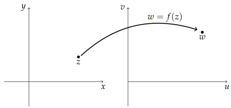
Letting \(z=x+i y\) and \(w=u+i v\), we can write the real and imaginary parts of \(f(z)\): \[w=f(z)=f(x+i y)=u(x, y)+i v(x, y) .\nonumber \] We see that one can view this function as a function of \(z\) or a function of \(x\) and \(y\). Often, we have an interest in writing out the real and imaginary parts of the function, \(u(x, y)\) and \(v(x, y)\), which are functions of two real variables, \(x\) and \(y\). We will look at several functions to determine the real and imaginary parts.
Find the real and imaginary parts of \(f(z)=z^{2}\).
Solution
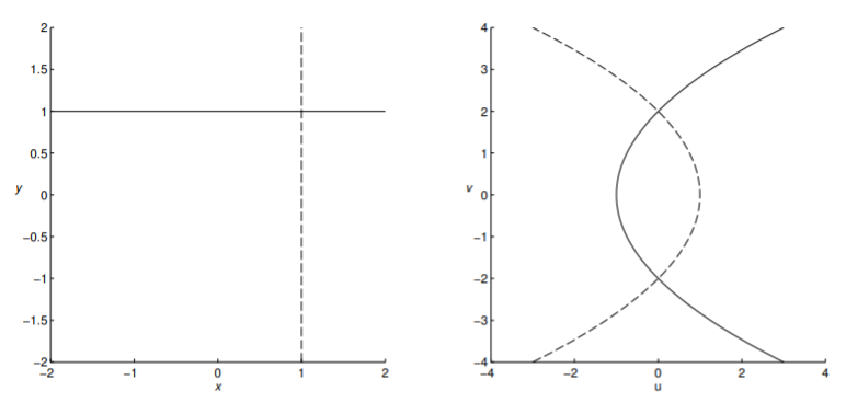
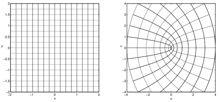
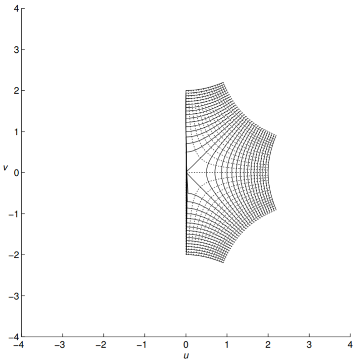
For example, we can look at the simple function \(f(z)=z^{2}\). It is a simple matter to determine the real and imaginary parts of this function. Namely, we have \[z^{2}=(x+i y)^{2}=x^{2}-y^{2}+2 i x y .\nonumber \] Therefore, we have that \[u(x, y)=x^{2}-y^{2}, \quad v(x, y)=2 x y .\nonumber \]
In Figure \(\PageIndex{2}\) we show how a grid in the z-plane is mapped by \(f(z)=z^{2}\) into the \(w\)-plane. For example, the horizontal line \(x=1\) is mapped to \(u(1, y)=1-y^{2}\) and \(v(1, y)=2 y\). Eliminating the "parameter" \(y\) between these two equations, we have \(u=1-v^{2} / 4\). This is a parabolic curve. Similarly, the horizontal line \(y=1\) results in the curve \(u=v^{2} / 4-1\).
If we look at several curves, \(x=\) const and \(y=\) const, then we get a family of intersecting parabolae, as shown in Figure \(\PageIndex{2}\).
Find the real and imaginary parts of \(f(z)=e^{z}\).
Solution
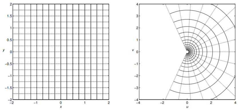
For this case, we make use of Euler’s Formula. \[\begin{align} e^{z} &=e^{x+i y}\nonumber \\ &=e^{x} e^{i y}\nonumber \\ &=e^{x}(\cos y+i \sin y) .\label{eq:1} \end{align}\] Thus, \(u(x, y)=e^{x} \cos y\) and \(v(x, y)=e^{x} \sin y .\) In Figure \(\PageIndex{4}\) we show how a grid in the \(z\)-plane is mapped by \(f(z)=e^{z}\) into the w-plane.
Find the real and imaginary parts of \(f(z)=z^{1 / 2}\).
Solution
We have that \[z^{1 / 2}=\sqrt{x^{2}+y^{2}}(\cos (\theta+k \pi)+i \sin (\theta+k \pi)), \quad k=0,1 .\label{eq:2}\] Thus, \[u=|z| \cos (\theta+k \pi), u=|z| \cos (\theta+k \pi)\nonumber \] for \(|z|=\sqrt{x^{2}+y^{2}}\) and \(\theta=\tan ^{-1}(y / x)\). For each \(k\)-value one has a different surface and curves of constant \(\theta\) give \(u / v=c_{1}\), and curves of constant nonzero complex modulus give concentric circles, \(u^{2}+v^{2}=c_{2}\), for \(c_{1}\) and \(c_{2}\) constants.
Find the real and imaginary parts of \(f(z)=\ln z\).
Solution
In this case we make use of the polar form of a complex number, \(z=r e^{i \theta}\). Our first thought would be to simply compute \[\ln z=\ln r+i \theta \text {. }\nonumber \] However, the natural logarithm is multivalued, just like the square root function. Recalling that \(e^{2 \pi i k}=1\) for \(k\) an integer, we have \(z=r e^{i(\theta+2 \pi k)}\). Therefore, \[\ln z=\ln r+i(\theta+2 \pi k), \quad k=\text { integer. }\nonumber\]
The natural logarithm is a multivalued function. In fact there are an infinite number of values for a given \(z\). Of course, this contradicts the definition of a function that you were first taught.
Thus, one typically will only report the principal value, \(\log z=\ln r+i \theta\), for \(\theta\) restricted to some interval of length \(2 \pi\), such as \([0,2 \pi)\). In order to account for the multivaluedness, one introduces a way to extend the complex plane so as to include all of the branches. This is done by assigning a plane to each branch, using (branch) cuts along lines, and then gluing the planes together at the branch cuts to form what is called a Riemann surface. We will not elaborate upon this any further here and refer the interested reader to more advanced texts. Comparing the multivalued logarithm to the principal value logarithm, we have \[\ln z=\log z+2 n \pi i .\nonumber \]
We should not that some books use \(\log z\) instead of \(\ln z\). It should not be confused with the common logarithm.
Complex Domain Coloring
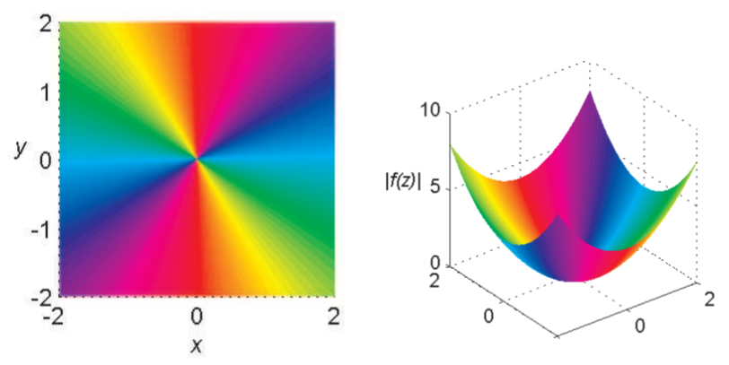
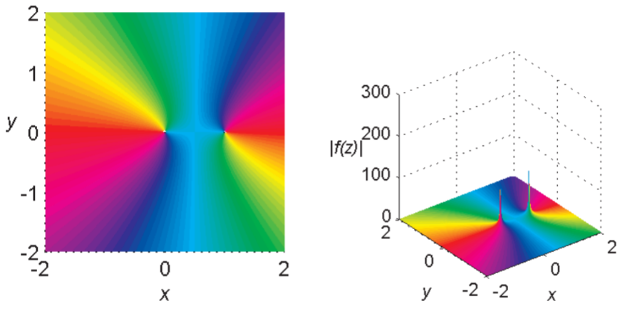
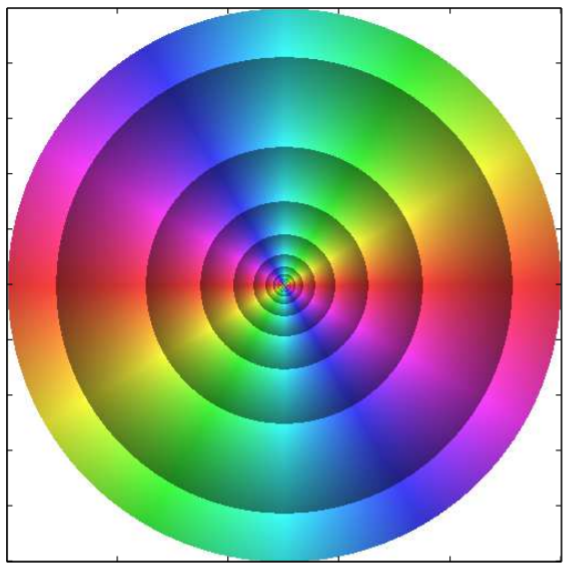
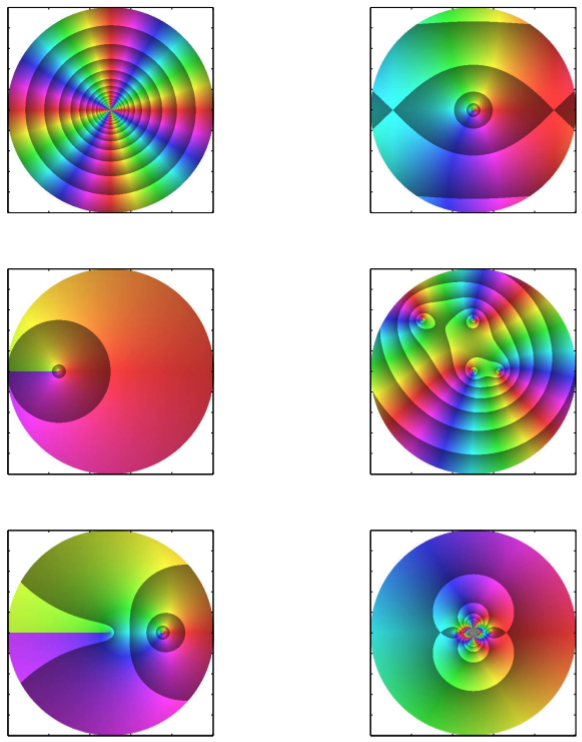
Another method for visualizing complex functions is domain coloring. The idea was described by Frank A. Farris. There are a few approaches to this method. The main idea is that one colors each point of the \(z\)-plane (the domain) according to \(\text{arg}(z)\) as shown in Figure \(\PageIndex{6}\). The modulus, \(|f(z)|\) is then plotted as a surface. Examples are shown for \(f(z)=z^2\) in Figure \(\PageIndex{7}\) and \(f(z)=1/z(1-z)\) in Figure \(\PageIndex{8}\).
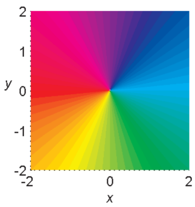
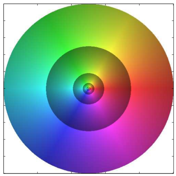
We would like to put all of this information in one plot. We can do this by adjusting the brightness of the colored domain by using the modulus of the function. In the plots that follow we use the fractional part of \(\ln |z|\). In Figure \(\PageIndex{9}\) we show the effect for the \(z\)-plane using \(f(z)=z\). In the figures that follow we look at several other functions. In these plots we have chosen to view the functions in a circular window.
One can see the rich behavior hidden in these figures. As you progress in your reading, especially after the next chapter, you should return to these figures and locate the zeros, poles, branch points and branch cuts. A search online will lead you to other colorings and superposition of the \(u v\) grid on these figures.
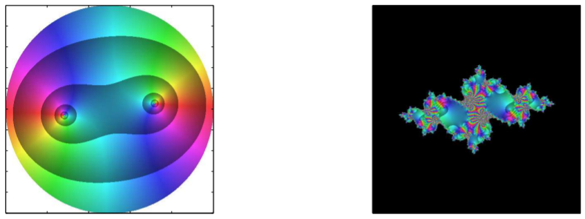
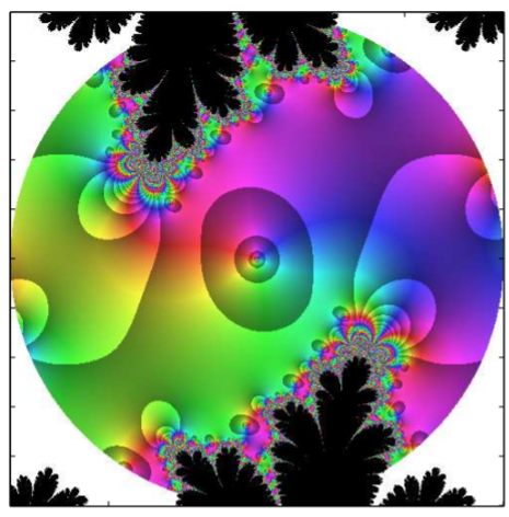
As a final picture, we look at iteration in the complex plane. Consider the function \(f(z) = z^2 − 0.75 − 0.2i\). Interesting figures result when studying the iteration in the complex plane. In Figure \(\PageIndex{12}\) we show \(f(z)\) and \(f^{20}(z)\), which is the iteration of \(f\) twenty times. It leads to an interesting coloring. What happens when one keeps iterating? Such iterations lead to the study of Julia and Mandelbrot sets. In Figure \(\PageIndex{13}\) we show six iterations of \(f(z) = (1 − i/2) \sin x\).
The following code was used in MATLAB to produce these figures.
fn = @(x) (1-i/2)*sin(x);
xmin=-2; xmax=2; ymin=-2; ymax=2;
Nx=500;
Ny=500;
x=linspace(xmin,xmax,Nx);
y=linspace(ymin,ymax,Ny);
[X,Y] = meshgrid(x,y); z = complex(X,Y);
tmp=z; for n=1:6
    tmp = fn(tmp);
end Z=tmp;
XX=real(Z);
YY=imag(Z);
R2=max(max(X.^2));
R=max(max(XX.^2+YY.^2));

circle(:,:,1) = X.^2+Y.^2 < R2;
circle(:,:,2)=circle(:,:,1);
circle(:,:,3)=circle(:,:,1);

addcirc(:,:,1)=circle(:,:,1)==0;
addcirc(:,:,2)=circle(:,:,1)==0;
addcirc(:,:,3)=circle(:,:,1)==0;

warning off MATLAB:divideByZero;
hsvCircle=ones(Nx,Ny,3);
hsvCircle(:,:,1)=atan2(YY,XX)*180/pi+(atan2(YY,XX)*180/pi<0)*360;
hsvCircle(:,:,1)=hsvCircle(:,:,1)/360; lgz=log(XX.^2+YY.^2)/2;
hsvCircle(:,:,2)=0.75; hsvCircle(:,:,3)=1-(lgz-floor(lgz))/2;
hsvCircle(:,:,1) = flipud((hsvCircle(:,:,1)));

hsvCircle(:,:,2) = flipud((hsvCircle(:,:,2)));

hsvCircle(:,:,3) =flipud((hsvCircle(:,:,3)));

rgbCircle=hsv2rgb(hsvCircle);
rgbCircle=rgbCircle.*circle+addcirc;
image(rgbCircle) axis square set(gca,’XTickLabel’,{}) set(gca,’YTickLabel’,{})