9.3: Exponential Fourier Transform

Both the trigonometric and complex exponential Fourier series provide us with representations of a class of functions of finite period in terms of sums over a discrete set of frequencies. In particular, for functions defined on \(x \in[-L, L]\), the period of the Fourier series representation is \(2 L\). We can write the arguments in the exponentials, \(e^{-i n \pi x / L}\), in terms of the angular frequency, \(\omega_{n}=n \pi / L\), as \(e^{-i \omega_{n} x}\). We note that the frequencies, \(v_{n}\), are then defined through \(\omega_{n}=2 \pi v_{n}=\frac{n \pi}{L}\). Therefore, the complex exponential series is seen to be a sum over a discrete, or countable, set of frequencies.

We would now like to extend the finite interval to an infinite interval, \(x \in(-\infty, \infty)\), and to extend the discrete set of (angular) frequencies to a continuous range of frequencies, \(\omega \in(-\infty, \infty)\). One can do this rigorously. It amounts to letting \(L\) and \(n\) get large and keeping \(\frac{n}{L}\) fixed.

We first define \(\Delta \omega=\frac{\pi}{L}\), so that \(\omega_{n}=n \Delta \omega\). Inserting the Fourier coefficients (9.2.12) into Equation (9.2.11), we have \[\begin{align} f(x) & \sim \sum_{n=-\infty}^{\infty} c_{n} e^{-i n \pi x / L}\nonumber \\ &=\sum_{n=-\infty}^{\infty}\left(\frac{1}{2 L} \int_{-L}^{L} f(\xi) e^{i n \pi \tilde{\zeta} / L} d \xi\right) e^{-i n \pi x / L}\nonumber \\ &=\sum_{n=-\infty}^{\infty}\left(\frac{\Delta \omega}{2 \pi} \int_{-L}^{L} f(\xi) e^{i \omega_{n} \tilde{}} d \xi\right) e^{-i \omega_{n} x} .\label{eq:1} \end{align}\]

Now, we let \(L\) get large, so that \(\Delta \omega\) becomes small and \(\omega_{n}\) approaches the angular frequency \(\omega\). Then, \[\begin{align} f(x) & \sim \lim _{\Delta \omega \rightarrow 0, L \rightarrow \infty} \frac{1}{2 \pi} \sum_{n=-\infty}^{\infty}\left(\int_{-L}^{L} f(\xi) e^{i \omega_{n} \tilde{\zeta}} d \xi\right) e^{-i \omega_{n} x} \Delta \omega\nonumber \\ &=\frac{1}{2 \pi} \int_{-\infty}^{\infty}\left(\int_{-\infty}^{\infty} f(\xi) e^{i \omega \zeta} d \xi\right) e^{-i \omega x} d \omega .\label{eq:2} \end{align}\]

Note

Definitions of the Fourier transform and the inverse Fourier transform.

Looking at this last result, we formally arrive at the definition of the Fourier transform. It is embodied in the inner integral and can be written as \[F[f]=\hat{f}(\omega)=\int_{-\infty}^{\infty} f(x) e^{i \omega x} d x\label{eq:3}\] This is a generalization of the Fourier coefficients (9.2.12).

Once we know the Fourier transform, \(\hat{f}(\omega)\), then we can reconstruct the original function, \(f(x)\), using the inverse Fourier transform, which is given by the outer integration, \[F^{-1}[\hat{f}]=f(x)=\frac{1}{2 \pi} \int_{-\infty}^{\infty} \hat{f}(\omega) e^{-i \omega x} d \omega .\label{eq:4}\] We note that it can be proven that the Fourier transform exists when \(f(x)\) is absolutely integrable, i.e., \[\int_{-\infty}^{\infty}|f(x)| d x<\infty .\nonumber \] Such functions are said to be \(L_{1}\).

We combine these results below, defining the Fourier and inverse Fourier transforms and indicating that they are inverse operations of each other. We will then prove the first of the equations, \(\eqref{eq:7}\). [The second equation, \(\eqref{eq:8}\), follows in a similar way.]

Note

The Fourier transform and inverse Fourier transform are inverse operations. Defining the Fourier transform as \[F[f]=\hat{f}(\omega )=\int_{-\infty}^\infty f(x)e^{j\omega x}dx.\label{eq:5}\] and the inverse Fourier transform as \[F^{-1}[\hat{f}]=f(x)=\frac{1}{2\pi}\int_{-\infty}^\infty \hat{f}(\omega )e^{-i\omega x}d\omega .\label{eq:6}\] then \[F^{-1}[F[f]]=f(x)\label{eq:7}\] and \[F[F^{-1}[\hat{f}]]=\hat{f}(\omega ).\label{eq:8}\]

Proof \(\PageIndex{1}\)

The proof is carried out by inserting the definition of the Fourier transform, \(\eqref{eq:5}\), into the inverse transform definition, \(\eqref{eq:6}\), and then interchanging the orders of integration. Thus, we have \[\begin{align}F^{-1}[F[f]]&=\frac{1}{2\pi}\int_{-\infty}^\infty F[f]e^{-i\omega x}d\omega\nonumber \\ &=\frac{1}{2\pi}\int_{-\infty}^\infty \left[\int_{-\infty}^\infty f(\xi )e^{i\omega\xi}d\xi\right]e^{-i\omega x}d\omega\nonumber \\ &=\frac{1}{2\pi}\int_{-\infty}^\infty \int_{-\infty}^\infty f(\xi )e^{i\omega (\xi -x)}d\xi d\omega\nonumber \\ &=\frac{1}{2\pi}\int_{-\infty}^\infty \left[\int_{-\infty}^\infty e^{i\omega (\xi -x)}d\omega\right] f(\xi )d\xi .\label{eq:9}\end{align}\]

In order to complete the proof, we need to evaluate the inside integral, which does not depend upon \(f(x)\). This is an improper integral, so we first define \[D_\Omega (x)=\int_{-\Omega}^\Omega e^{i\omega x}d\omega\nonumber\] and compute the inner integral as \[\int_{-\infty}^\infty e^{i\omega (\xi -x)}d\omega =\lim_{\Omega\to\infty}D_\Omega (\xi -x).\nonumber\]

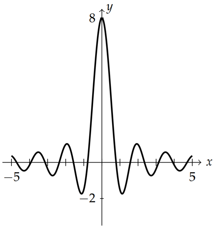
We can compute \(D_\Omega (x)\). A simple evaluation yields \[\begin{align}D_\Omega (x)&=\int_{-\Omega}^\Omega e^{-\omega x}d\omega\nonumber \\ &=\left.\frac{e^{i\omega x}}{ix}\right|_{-\infty}^\infty\nonumber \\ &=\frac{e^{ix\Omega}-e^{-ix\Omega}}{2ix}\nonumber \\ &=\frac{2\sin x\Omega}{x}.\label{eq:10}\end{align}\]

A plot of this function is in Figure \(\PageIndex{1}\) for \(\Omega=4\). For large \(\Omega\) the peak grows and the values of \(D_{\Omega}(x)\) for \(x \neq 0\) tend to zero as shown in Figure \(\PageIndex{2}\). In fact, as \(x\) approaches \(0, D_{\Omega}(x)\) approaches \(2 \Omega\). For \(x \neq 0\), the \(D_{\Omega}(x)\) function tends to zero.

Figure \(\PageIndex{1}\): A plot of the function \(D_{\Omega}(x)\) for \(\Omega=4\).

Figure \(\PageIndex{2}\): A plot of the function \(D_{\Omega}(x)\) for \(\Omega=40\).

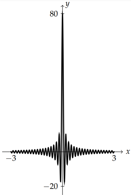
We further note that \[\lim _{\Omega \rightarrow \infty} D_{\Omega}(x)=0, \quad x \neq 0,\nonumber \] and \(\lim _{\Omega \rightarrow \infty} D_{\Omega}(x)\) is infinite at \(x=0\). However, the area is constant for each \(\Omega\). In fact, \[\int_{-\infty}^{\infty} D_{\Omega}(x) d x=2 \pi .\nonumber \] We can show this by recalling the computation in Example 8.5.30, \[\int_{-\infty}^{\infty} \frac{\sin x}{x} d x=\pi\nonumber \] Then, \[\begin{align} \int_{-\infty}^{\infty} D_{\Omega}(x) d x &=\int_{-\infty}^{\infty} \frac{2 \sin x \Omega}{x} d x\nonumber \\ &=\int_{-\infty}^{\infty} 2 \frac{\sin y}{y} d y\nonumber \\ &=2 \pi\label{eq:11} \end{align}\]

Another way to look at \(D_{\Omega}(x)\) is to consider the sequence of functions \(f_n(x)=\frac{\sin n x}{\pi x}, n=1,2, \ldots\) Then we have shown that this sequence of functions satisfies the two properties, \[\lim _{n \rightarrow \infty} f_{n}(x)=0, \quad x \neq 0,\nonumber \] \[\int_{-\infty}^{\infty} f_{n}(x) d x=1 .\nonumber \] This is a key representation of such generalized functions. The limiting value vanishes at all but one point, but the area is finite.

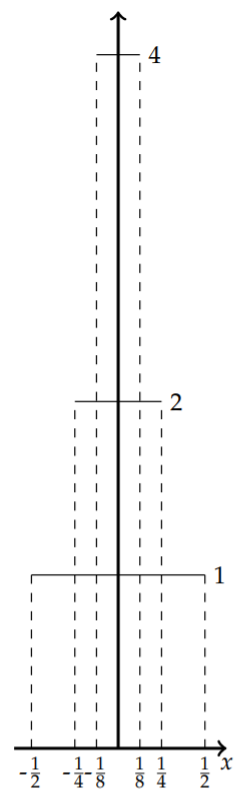
Such behavior can be seen for the limit of other sequences of functions. For example, consider the sequence of functions \[f_{n}(x)=\left\{\begin{array}{lc} 0, & |x|>\frac{1}{n}, \\ \frac{n}{2}, & |x|<\leq \text { frac1n } . \end{array}\right.\nonumber \] This is a sequence of functions as shown in Figure \(\PageIndex{3}\). As \(n \rightarrow \infty\), we find the limit is zero for \(x \neq 0\) and is infinite for \(x=0\). However, the area under each member of the sequences is one. Thus, the limiting function is zero at most points but has area one.

Figure \(\PageIndex{3}\): A plot of the functions \(f_{n}(x)\) for \(n=2,4,8\).

The limit is not really a function. It is a generalized function. It is called the Dirac delta function, which is defined by

1. \(\delta(x)=0 \text { for } x \neq 0 \text {. }\)
2. \(\int_{-\infty}^{\infty} \delta(x) d x=1 \text {. }\)

Before returning to the proof that the inverse Fourier transform of the Fourier transform is the identity, we state one more property of the Dirac delta function, which we will prove in the next section. Namely, we will show that \[\int_{-\infty}^{\infty} \delta(x-a) f(x) d x=f(a) .\nonumber \]

Returning to the proof, we now have that \[\int_{-\infty}^{\infty} e^{i \omega(\xi-x)} d \omega=\lim _{\Omega \rightarrow \infty} D_{\Omega}(\xi-x)=2 \pi \delta(\xi-x) .\nonumber \]

Inserting this into \(\eqref{eq:9}\), we have \[\begin{align} F^{-1}[F[f]] &=\frac{1}{2 \pi} \int_{-\infty}^{\infty}\left[\int_{-\infty}^{\infty} e^{i \omega(\xi-x)} d \omega\right] f(\xi) d \xi .\nonumber \\ &=\frac{1}{2 \pi} \int_{-\infty}^{\infty} 2 \pi \delta(\xi-x) f(\xi) d \xi .\nonumber \\ &=f(x) .\label{eq:12} \end{align}\] Thus, we have proven that the inverse transform of the Fourier transform of \(f\) is \(f\).