9.10: The Inverse Laplace Transform
- Page ID
- 90979

\( \newcommand{\vecs}[1]{\overset { \scriptstyle \rightharpoonup} {\mathbf{#1}} } \)
\( \newcommand{\vecd}[1]{\overset{-\!-\!\rightharpoonup}{\vphantom{a}\smash {#1}}} \)
\( \newcommand{\dsum}{\displaystyle\sum\limits} \)
\( \newcommand{\dint}{\displaystyle\int\limits} \)
\( \newcommand{\dlim}{\displaystyle\lim\limits} \)
\( \newcommand{\id}{\mathrm{id}}\) \( \newcommand{\Span}{\mathrm{span}}\)
( \newcommand{\kernel}{\mathrm{null}\,}\) \( \newcommand{\range}{\mathrm{range}\,}\)
\( \newcommand{\RealPart}{\mathrm{Re}}\) \( \newcommand{\ImaginaryPart}{\mathrm{Im}}\)
\( \newcommand{\Argument}{\mathrm{Arg}}\) \( \newcommand{\norm}[1]{\| #1 \|}\)
\( \newcommand{\inner}[2]{\langle #1, #2 \rangle}\)
\( \newcommand{\Span}{\mathrm{span}}\)
\( \newcommand{\id}{\mathrm{id}}\)
\( \newcommand{\Span}{\mathrm{span}}\)
\( \newcommand{\kernel}{\mathrm{null}\,}\)
\( \newcommand{\range}{\mathrm{range}\,}\)
\( \newcommand{\RealPart}{\mathrm{Re}}\)
\( \newcommand{\ImaginaryPart}{\mathrm{Im}}\)
\( \newcommand{\Argument}{\mathrm{Arg}}\)
\( \newcommand{\norm}[1]{\| #1 \|}\)
\( \newcommand{\inner}[2]{\langle #1, #2 \rangle}\)
\( \newcommand{\Span}{\mathrm{span}}\) \( \newcommand{\AA}{\unicode[.8,0]{x212B}}\)
\( \newcommand{\vectorA}[1]{\vec{#1}} % arrow\)
\( \newcommand{\vectorAt}[1]{\vec{\text{#1}}} % arrow\)
\( \newcommand{\vectorB}[1]{\overset { \scriptstyle \rightharpoonup} {\mathbf{#1}} } \)
\( \newcommand{\vectorC}[1]{\textbf{#1}} \)
\( \newcommand{\vectorD}[1]{\overrightarrow{#1}} \)
\( \newcommand{\vectorDt}[1]{\overrightarrow{\text{#1}}} \)
\( \newcommand{\vectE}[1]{\overset{-\!-\!\rightharpoonup}{\vphantom{a}\smash{\mathbf {#1}}}} \)
\( \newcommand{\vecs}[1]{\overset { \scriptstyle \rightharpoonup} {\mathbf{#1}} } \)
\(\newcommand{\longvect}{\overrightarrow}\)
\( \newcommand{\vecd}[1]{\overset{-\!-\!\rightharpoonup}{\vphantom{a}\smash {#1}}} \)
\(\newcommand{\avec}{\mathbf a}\) \(\newcommand{\bvec}{\mathbf b}\) \(\newcommand{\cvec}{\mathbf c}\) \(\newcommand{\dvec}{\mathbf d}\) \(\newcommand{\dtil}{\widetilde{\mathbf d}}\) \(\newcommand{\evec}{\mathbf e}\) \(\newcommand{\fvec}{\mathbf f}\) \(\newcommand{\nvec}{\mathbf n}\) \(\newcommand{\pvec}{\mathbf p}\) \(\newcommand{\qvec}{\mathbf q}\) \(\newcommand{\svec}{\mathbf s}\) \(\newcommand{\tvec}{\mathbf t}\) \(\newcommand{\uvec}{\mathbf u}\) \(\newcommand{\vvec}{\mathbf v}\) \(\newcommand{\wvec}{\mathbf w}\) \(\newcommand{\xvec}{\mathbf x}\) \(\newcommand{\yvec}{\mathbf y}\) \(\newcommand{\zvec}{\mathbf z}\) \(\newcommand{\rvec}{\mathbf r}\) \(\newcommand{\mvec}{\mathbf m}\) \(\newcommand{\zerovec}{\mathbf 0}\) \(\newcommand{\onevec}{\mathbf 1}\) \(\newcommand{\real}{\mathbb R}\) \(\newcommand{\twovec}[2]{\left[\begin{array}{r}#1 \\ #2 \end{array}\right]}\) \(\newcommand{\ctwovec}[2]{\left[\begin{array}{c}#1 \\ #2 \end{array}\right]}\) \(\newcommand{\threevec}[3]{\left[\begin{array}{r}#1 \\ #2 \\ #3 \end{array}\right]}\) \(\newcommand{\cthreevec}[3]{\left[\begin{array}{c}#1 \\ #2 \\ #3 \end{array}\right]}\) \(\newcommand{\fourvec}[4]{\left[\begin{array}{r}#1 \\ #2 \\ #3 \\ #4 \end{array}\right]}\) \(\newcommand{\cfourvec}[4]{\left[\begin{array}{c}#1 \\ #2 \\ #3 \\ #4 \end{array}\right]}\) \(\newcommand{\fivevec}[5]{\left[\begin{array}{r}#1 \\ #2 \\ #3 \\ #4 \\ #5 \\ \end{array}\right]}\) \(\newcommand{\cfivevec}[5]{\left[\begin{array}{c}#1 \\ #2 \\ #3 \\ #4 \\ #5 \\ \end{array}\right]}\) \(\newcommand{\mattwo}[4]{\left[\begin{array}{rr}#1 \amp #2 \\ #3 \amp #4 \\ \end{array}\right]}\) \(\newcommand{\laspan}[1]{\text{Span}\{#1\}}\) \(\newcommand{\bcal}{\cal B}\) \(\newcommand{\ccal}{\cal C}\) \(\newcommand{\scal}{\cal S}\) \(\newcommand{\wcal}{\cal W}\) \(\newcommand{\ecal}{\cal E}\) \(\newcommand{\coords}[2]{\left\{#1\right\}_{#2}}\) \(\newcommand{\gray}[1]{\color{gray}{#1}}\) \(\newcommand{\lgray}[1]{\color{lightgray}{#1}}\) \(\newcommand{\rank}{\operatorname{rank}}\) \(\newcommand{\row}{\text{Row}}\) \(\newcommand{\col}{\text{Col}}\) \(\renewcommand{\row}{\text{Row}}\) \(\newcommand{\nul}{\text{Nul}}\) \(\newcommand{\var}{\text{Var}}\) \(\newcommand{\corr}{\text{corr}}\) \(\newcommand{\len}[1]{\left|#1\right|}\) \(\newcommand{\bbar}{\overline{\bvec}}\) \(\newcommand{\bhat}{\widehat{\bvec}}\) \(\newcommand{\bperp}{\bvec^\perp}\) \(\newcommand{\xhat}{\widehat{\xvec}}\) \(\newcommand{\vhat}{\widehat{\vvec}}\) \(\newcommand{\uhat}{\widehat{\uvec}}\) \(\newcommand{\what}{\widehat{\wvec}}\) \(\newcommand{\Sighat}{\widehat{\Sigma}}\) \(\newcommand{\lt}{<}\) \(\newcommand{\gt}{>}\) \(\newcommand{\amp}{&}\) \(\definecolor{fillinmathshade}{gray}{0.9}\)Until this point we have seen that the inverse Laplace transform can be found by making use of Laplace transform tables and properties of Laplace transforms. This is typically the way Laplace transforms are taught and used in a differential equations course. One can do the same for Fourier transforms. However, in the case of Fourier transforms we introduced an inverse transform in the form of an integral. Does such an inverse integral transform exist for the Laplace transform? Yes, it does! In this section we will derive the inverse Laplace transform integral and show how it is used.
We begin by considering a causal function \(f(t)\) which vanishes for \(t<0\) and define the function \(g(t)=f(t) e^{-c t}\) with \(c>0\). For \(g(t)\) absolutely integrable,
\[\int_{-\infty}^{\infty}|g(t)| d t=\int_{0}^{\infty}|f(t)| e^{-c t} d t<\infty,\nonumber \]
we can write the Fourier transform,
\[\hat{g}(\omega)=\int_{-\infty}^{\infty} g(t) e^{i \omega t} d t=\int_{0}^{\infty} f(t) e^{i \omega t-c t} d t\nonumber \]
and the inverse Fourier transform,
\[g(t)=f(t) e^{-c t}=\frac{1}{2 \pi} \int_{-\infty}^{\infty} \hat{g}(\omega) e^{-i \omega t} d \omega .\nonumber \]
Multiplying by \(e^{c t}\) and inserting \(\hat{g}(\omega)\) into the integral for \(g(t)\), we find
\[f(t)=\frac{1}{2 \pi} \int_{-\infty}^{\infty} \int_{0}^{\infty} f(\tau) e^{(i \omega-c) \tau} d \tau e^{-(i \omega-c) t} d \omega .\nonumber \]
Letting \(s=c-i \omega(\) so \(d \omega=i d s)\), we have
\[f(t)=\frac{i}{2 \pi} \int_{c+i \infty}^{c-i \infty} \int_{0}^{\infty} f(\tau) e^{-s \tau} d \tau e^{s t} d s\nonumber \]
Note that the inside integral is simply \(F(s)\). So, we have
\[f(t)=\frac{1}{2 \pi i} \int_{c-i \infty}^{c+i \infty} F(s) e^{s t} d s .\label{eq:1} \]
The integral in the last equation is the inverse Laplace transform, called the Bromwich integral and is named after Thomas John I’Anson Bromwich (1875-1929). This inverse transform is not usually covered in differential equations courses because the integration takes place in the complex plane. This integral is evaluated along a path in the complex plane called the Bromwich contour. The typical way to compute this integral is to first chose \(c\) so that all poles are to the left of the contour. This guarantees that \(f(t)\) is of exponential type. The contour is closed a semicircle enclosing all of the poles. One then relies on a generalization of Jordan’s lemma to the second and third quadrants.\(^{1}\)
Closing the contour to the left of the contour can be reasoned in a manner similar to what we saw in Jordan’s Lemma. Write the exponential as \(e^{s t}=\) \(e^{\left(s_{R}+i s_{I}\right) t}=e^{s_{R} t} e^{i s_{l} t}\). The second factor is an oscillating factor and the growth in the exponential can only come from the first factor. In order for the exponential to decay as the radius of the semicircle grows, \(s_{R} t<0\). Since \(t>0\), we need \(s<0\) which is done by closing the contour to the left. If \(t<0\), then the contour to the right would enclose no singularities and preserve the causality of \(f(t)\).
Find the inverse Laplace transform of \(F(s)=\frac{1}{s(s+1)}\).
Solution
The integral we have to compute is
\[f(t)=\frac{1}{2 \pi i} \int_{c-i \infty}^{c+i \infty} \frac{e^{s t}}{s(s+1)} d s\nonumber \]
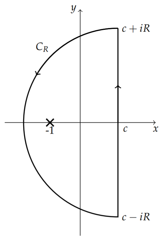
This integral has poles at \(s=0\) and \(s=-1\). The contour we will use is shown in Figure \(\PageIndex{1}\). We enclose the contour with a semicircle to the left of the path in the complex s-plane. One has to verify that the integral over the semicircle vanishes as the radius goes to infinity. Assuming that we have done this, then the result is simply obtained as \(2 \pi i\) times the sum of the residues. The residues in this case are:
\[\operatorname{Res}\left[\frac{e^{z t}}{z(z+1)} ; z=0\right]=\lim _{z \rightarrow 0} \frac{e^{z t}}{(z+1)}=1\nonumber \]
and
\[\operatorname{Res}\left[\frac{e^{z t}}{z(z+1)} ; z=-1\right]=\lim _{z \rightarrow-1} \frac{e^{z t}}{z}=-e^{-t} .\nonumber \]
Therefore, we have
\[f(t)=2 \pi i\left[\frac{1}{2 \pi i}(1)+\frac{1}{2 \pi i}\left(-e^{-t}\right)\right]=1-e^{-t} .\nonumber \]
We can verify this result using the Convolution Theorem or using a partial fraction decomposition. The latter method is simplest. We note that
\[\frac{1}{s(s+1)}=\frac{1}{s}-\frac{1}{s+1} \text {. }\nonumber \]
The first term leads to an inverse transform of 1 and the second term gives \(e^{-t}\). So,
\[\mathcal{L}^{-1}\left[\frac{1}{s}-\frac{1}{s+1}\right]=1-e^{-t} .\nonumber \]
Thus, we have verified the result from doing contour integration.
Find the inverse Laplace transform of \(F(s)=\frac{1}{s\left(1+e^{s}\right)}\).
Solution
In this case, we need to compute
\[f(t)=\frac{1}{2 \pi i} \int_{c-i \infty}^{c+i \infty} \frac{e^{s t}}{s\left(1+e^{s}\right)} d s .\nonumber \]
This integral has poles at complex values of s such that \(1+e^{s}=0\), or \(e^{s}=-1\). Letting \(s=x+i y\), we see that
\[e^{s}=e^{x+i y}=e^{x}(\cos y+i \sin y)=-1 .\nonumber \]
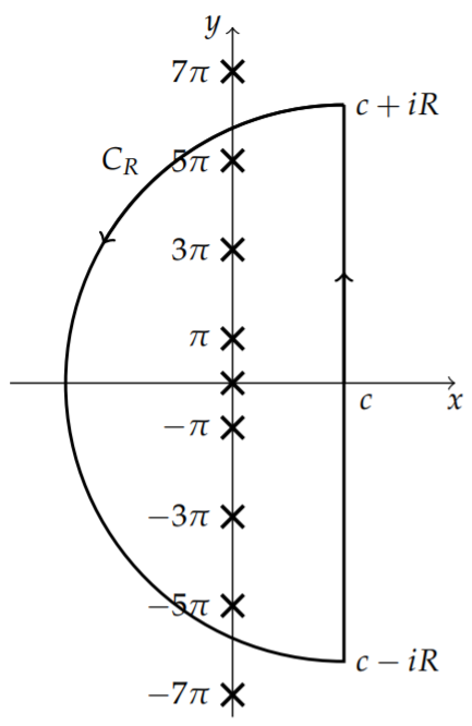
We see \(x=0\) and \(y\) satisfies \(\cos y=-1\) and \(\sin y=0\). Therefore, \(y=n \pi\) for \(n\) an odd integer. Therefore, the integrand has an infinite number of simple poles at \(s=n \pi i, n=\pm 1, \pm 3, \ldots\). It also has a simple pole at \(s=0\).
In Figure \(\PageIndex{2}\) we indicate the poles. We need to compute the resides at each pole. At \(s=n \pi i\) we have
\[\begin{align} \operatorname{Res}\left[\frac{e^{st}}{s(1+e^s)};\: s=n\pi i\right]&=\lim_{s\to n\pi i}(s-n\pi i)\frac{e^{st}}{s(1+e^s)}\nonumber \\ &=\lim_{s\to n\pi i}\frac{e^{st}}{se^s}\nonumber \\ &=-\frac{e^{n\pi it}}{n\pi i},\quad n\text{ odd}.\label{eq:2}\end{align} \]
At \(s=0\), the residue is
\[\operatorname{Res}\left[\frac{e^{s t}}{s\left(1+e^{s}\right)} ; s=0\right]=\lim _{s \rightarrow 0} \frac{e^{s t}}{1+e^{s}}=\frac{1}{2} .\nonumber \]
Summing the residues and noting the exponentials for \(\pm n\) can be combined to form sine functions, we arrive at the inverse transform.
\[\begin{align} f(t) &=\frac{1}{2}-\sum_{n \text { odd }} \frac{e^{n \pi i t}}{n \pi i}\nonumber \\ &=\frac{1}{2}-2 \sum_{k=1}^{\infty} \frac{\sin (2 k-1) \pi t}{(2 k-1) \pi} .\label{eq:3} \end{align} \]
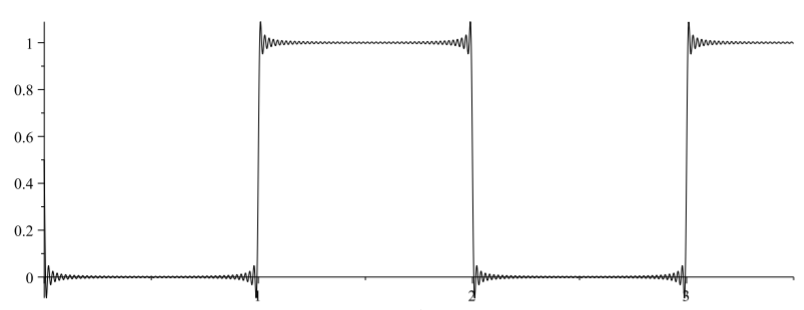
The series in this example might look familiar. It is a Fourier sine series with odd harmonics whose amplitudes decay like \(1 / n\). It is a vertically shifted square wave. In fact, we had computed the Laplace transform of a general square wave in Example 9.8.7.
In that example we found
\[\begin{align} \mathcal{L}\left[\sum_{n=0}^{\infty}[H(t-2 n a)-H(t-(2 n+1) a)]\right] &=\frac{1-e^{-a s}}{s\left(1-e^{-2 a s}\right)}\nonumber \\ &=\frac{1}{s\left(1+e^{-a s}\right)} .\label{eq:4} \end{align} \]
In this example, one can show that
\[f(t)=\sum_{n=0}^{\infty}[H(t-2 n+1)-H(t-2 n)] .\nonumber \]
The reader should verify that this result is indeed the square wave shown in Figure \(\PageIndex{3}\).