
9.11: Transforms and Partial Differential Equations


- Last updated
- Sep 4, 2024
- Save as PDF

( \newcommand{\kernel}{\mathrm{null}\,}\)
As another application of the transforms, we will see that we can use transforms to solve some linear partial differential equations. We will first solve the one dimensional heat equation and the two dimensional Laplace equations using Fourier transforms. The transforms of the partial differential equations lead to ordinary differential equations which are easier to solve. The final solutions are then obtained using inverse transforms.
We could go further by applying a Fourier transform in space and a Laplace transform in time to convert the heat equation into an algebraic equation. We will also show that we can use a finite sine transform to solve nonhomogeneous problems on finite intervals. Along the way we will identify several Green’s functions.
Fourier Transform and the Heat Equation
We will first consider the solution of the heat equation on an infinite interval using Fourier transforms. The basic scheme has been discussed earlier and is outlined in Figure 9.11.1.
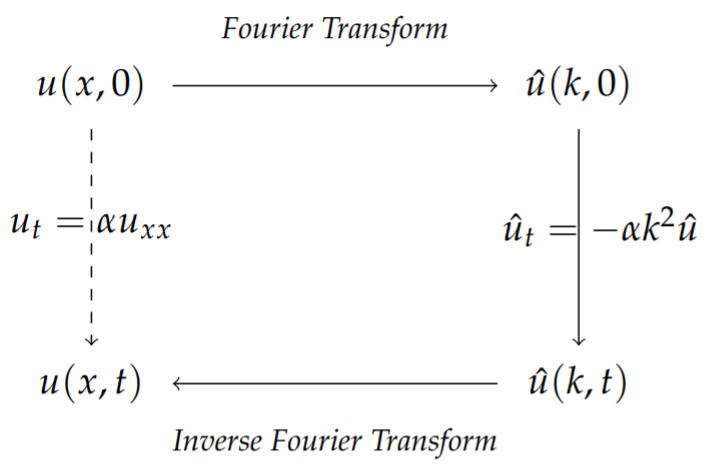
Consider the heat equation on the infinite line,
ut=αuxx,−∞<x<∞,t>0.u(x,0)=f(x),−∞<x<∞.
We can Fourier transform the heat equation using the Fourier transform of u(x,t),
F[u(x,t)]=ˆu(k,t)=∫∞−∞u(x,t)eikxdx
We need to transform the derivatives in the equation. First we note that
F[ut]=∫∞−∞∂u(x,t)∂teikxdx=∂∂t∫∞−∞u(x,t)eikxdx=∂ˆu(k,t)∂t
Assuming that lim|x|→∞u(x,t)=0 and lim|x|→∞ux(x,t)=0, then we also have that
F[uxx]=∫∞−∞∂2u(x,t)∂x2eikxdx=−k2ˆu(k,t)
Therefore, the heat equation becomes
∂ˆu(k,t)∂t=−αk2ˆu(k,t)
This is a first order differential equation which is readily solved as
ˆu(k,t)=A(k)e−αk2t
where A(k) is an arbitrary function of k. The inverse Fourier transform is
u(x,t)=12π∫∞−∞ˆu(k,t)e−ikxdk=12π∫∞−∞ˆA(k)e−αk2te−ikxdk
We can determine A(k) using the initial condition. Note that
F[u(x,0)]=ˆu(k,0)=∫∞−∞f(x)eikxdx.
But we also have from the solution,
u(x,0)=12π∫∞−∞ˆA(k)e−ikxdk.
Comparing these two expressions for ˆu(k,0), we see that
A(k)=F[f(x)].
We note that ˆu(k,t) is given by the product of two Fourier transforms, ˆu(k,t)=A(k)e−αk2t. So, by the Convolution Theorem, we expect that u(x,t) is the convolution of the inverse transforms,
u(x,t)=(f∗g)(x,t)=12π∫∞−∞f(ξ,t)g(x−ξ,t)dξ,
where
g(x,t)=F−1[e−αk2t]
In order to determine g(x,t), we need only recall Example 9.5.1. In that example we saw that the Fourier transform of a Gaussian is a Gaussian. Namely, we found that
F[e−ax2/2]=√2πae−k2/2a,
or,
F−1[√2πae−k2/2a]=e−ax2/2.
Applying this to the current problem, we have
g(x)=F−1[e−αk2t]=√παte−x2/4t.
Finally, we can write down the solution to the problem:
u(x,t)=(f∗g)(x,t)=∫∞−∞f(ξ,t)e−(x−ξ)2/4t√4παtdξ,
The function in the integrand,
K(x,t)=e−x2/4t√4παt
is called the heat kernel.
Laplace’s Equation on the Half Plane
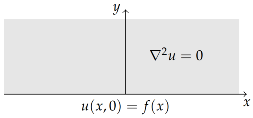
We consider a steady state solution in two dimensions. In particular, we look for the steady state solution, u(x,y), satisfying the two-dimensional Laplace equation on a semi-infinite slab with given boundary conditions as shown in Figure 9.11.2. The boundary value problem is given as
uxx+uyy=0,−∞<x<∞,y>0,u(x,0)=f(x),−∞<x<∞limy→∞u(x,y)=0,lim|x|→∞u(x,y)=0.
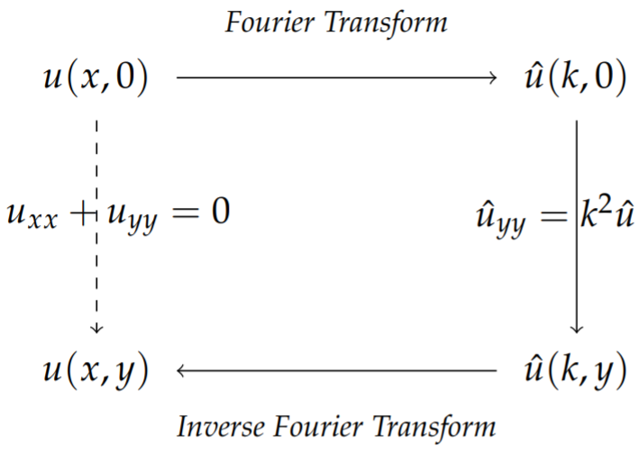
This problem can be solved using a Fourier transform of u(x,y) with respect to x. The transform scheme for doing this is shown in Figure 9.11.3. We begin by defining the Fourier transform
ˆu(k,y)=F[u]=∫∞−∞u(x,y)eikxdx.
We can transform Laplace’s equation. We first note from the properties of Fourier transforms that
F[∂2u∂x2]=−k2ˆu(k,y),
if lim|x|→∞u(x,y)=0 and lim|x|→∞ux(x,y)=0. Also,
F[∂2u∂y2]=∂2ˆu(k,y)∂y2.
Thus, the transform of Laplace’s equation gives ˆuyy=k2ˆu.
This is a simple ordinary differential equation. We can solve this equation using the boundary conditions. The general solution is
ˆu(k,y)=a(k)eky+b(k)e−ky.
Since limy→∞u(x,y)=0 and k can be positive or negative, we have that ˆu(k,y)=a(k)e−|k|y. The coefficient a(k) can be determined using the remaining boundary condition, u(x,0)=f(x). We find that a(k)=ˆf(k) since
a(k)=ˆu(k,0)=∫∞−∞u(x,0)eikxdx=∫∞−∞f(x)eikxdx=ˆf(k).
We have found that ˆu(k,y)=ˆf(k)e−|k|y. We can obtain the solution using the inverse Fourier transform,
u(x,t)=F−1[ˆf(k)e−|k|y].
We note that this is a product of Fourier transforms and use the Convolution Theorem for Fourier transforms. Namely, we have that a(k)=F[f] and e−|k|y=F[g] for g(x,y)=2yx2+y2. This last result is essentially proven in Problem 6.
Then, the Convolution Theorem gives the solution
u(x,y)=12π∫∞−∞f(ξ)g(x−ξ)dξ=12π∫∞−∞f(ξ)2y(x−ξ)2+y2dξ
We note for future use, that this solution is in the form
u(x,y)=∫∞−∞f(ξ)G(x,ξ;y,0)dξ,
where
G(x,ξ;y,0)=2yπ((x−ξ)2+y2)
is the Green’s function for this problem.
Heat Equation on Infinite Interval, Revisited
We will reconsider the initial value problem for the heat equation on an infinite interval,
ut=uxx,−∞<x<∞,t>0u(x,0)=f(x),−∞<x<∞.
We can apply both a Fourier and a Laplace transform to convert this to an algebraic problem. The general solution will then be written in terms of an initial value Green’s function as
u(x,t)=∫∞−∞G(x,t;ξ,0)f(ξ)dξ.
For the time dependence we can use the Laplace transform and for the spatial dependence we use the Fourier transform. These combined transforms lead us to define
ˆu(k,s)=F[L[u]]=∫∞−∞∫∞0u(x,t)e−steikxdtdx.
Applying this to the terms in the heat equation, we have
F[L[ut]]=sˆu(k,s)−F[u(x,0)]=sˆu(k,s)−ˆf(k)F[L[uxx]]=−k2ˆu(k,s).
Here we have assumed that
limt→∞u(x,t)e−st=0,lim|x|→∞u(x,t)=0,lim|x|→∞ux(x,t)=0.
Therefore, the heat equation can be turned into an algebraic equation for the transformed solution,
(s+k2)ˆu(k,s)=ˆf(k),
or
ˆu(k,s)=ˆf(k)s+k2.
The solution to the heat equation is obtained using the inverse transforms for both the Fourier and Laplace transform. Thus, we have
u(x,t)=F−1[L−1[ˆu]]=12π∫∞−∞(12πi∫c+∞c−i∞ˆf(k)s+k2estds)e−ikxdk.
Since the inside integral has a simple pole at s=−k2, we can compute the Bromwich integral by choosing c>−k2. Thus,
12πi∫c+∞c−i∞ˆf(k)s+k2estds=Res[ˆf(k)s+k2est;s=−k2]=e−k2tˆf(k).
Inserting this result into the solution, we have
u(x,t)=F−1[L−1[ˆu]]=12π∫∞−∞ˆf(k)e−k2te−ikxdk.
This solution is of the form
u(x,t)=F−1[ˆfˆg]
for ˆg(k)=e−k2t. So, by the Convolution Theorem for Fourier transforms, the solution is a convolution,
u(x,t)=∫∞−∞f(ξ)g(x−ξ)dξ
All we need is the inverse transform of ˆg(k).
We note that ˆg(k)=e−k2t is a Gaussian. Since the Fourier transform of a Gaussian is a Gaussian, we need only recall Example 9.5.1,
F[e−ax2/2]=√2πae−k2/2a.
Setting a=1/2t, this becomes
F[e−x2/4t]=√4πte−k2t.
So,
g(x)=F−1[e−k2t]=e−x2/4t√4πt
Inserting g(x) into the solution, we have
u(x,t)=1√4πt∫∞−∞f(ξ)e−(x−ξ)2/4tdξ=∫∞−∞G(x,t;ζ,0)f(ξ)dξ
Here we have identified the initial value Green’s function
G(x,t;ξ,0)=1√4πte−(x−ξ)2/4t.
Nonhomogeneous Heat Equation
We now consider the nonhomogeneous heat equation with homogeneous boundary conditions defined on a finite interval.
ut−kuxx=h(x,t),0≤x≤L,t>0u(0,t)=0,u(L,t)=0,t>0u(x,0)=f(x),0≤x≤
We know that when h(x,t)≡0 the solution takes the form
u(x,t)=∞∑n=1bnsinnπxL
So, when h(x,t)≠0, we might assume that the solution takes the form
u(x,t)=∞∑n=1bn(t)sinnπxL
where the b′n s are the finite Fourier sine transform of the desired solution,
bn(t)=Fs[u]=2L∫L0u(x,t)sinnπxLdx
Note that the finite Fourier sine transform is essentially the Fourier sine transform which we encountered in Section 3.4.
The idea behind using the finite Fourier Sine Transform is to solve the given heat equation by transforming the heat equation to a simpler equation for the transform, bn(t), solve for bn(t), and then do an inverse transform, i.e., insert the bn(t) ’s back into the series representation. This is depicted in Figure 9.11.4. Note that we had explored similar diagram earlier when discussing the use of transforms to solve differential equations.
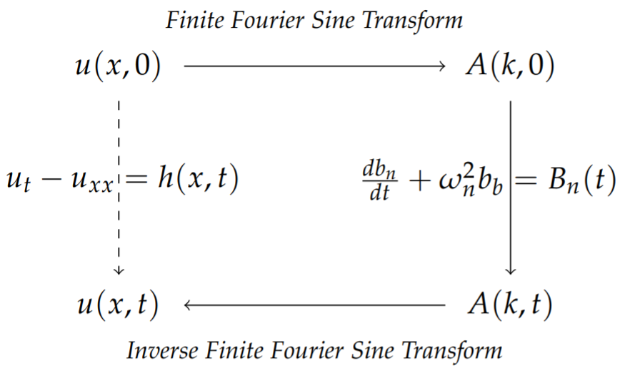
First, we need to transform the partial differential equation. The finite transforms of the derivative terms are given by
Fs[ut]=2L∫L0∂u∂t(x,t)sinnπxLdx=ddt(2L∫L0u(x,t)sinnπxLdx)=dbndt.
Fs[uxx]=2L∫L0∂2u∂x2(x,t)sinnπxLdx=[uxsinnπxL]L0−(nπL)2L∫L0∂u∂x(x,t)cosnπxLdx=−[nπLucosnπxL]L0−(nπL)22L∫L0u(x,t)sinnπxLdx=nπL[u(0,t)−u(L,0)cosnπ]−(nπL)2b2n=−ω2nb2n,
where ωn=nπL.
Furthermore, we define
Hn(t)=Fs[h]=2L∫L0h(x,t)sinnπxLdx.
Then, the heat equation is transformed to
dbndt+ω2nbn=Hn(t),n=1,2,3,….
This is a simple linear first order differential equation. We can supplement this equation with the initial condition
bn(0)=2L∫L0u(x,0)sinnπxLdx.
The differential equation for bn is easily solved using the integrating factor, μ(t)=eω2nt. Thus,
ddt(eω2ntbn(t))=Hn(t)eω2nt
and the solution is
bn(t)=bn(0)e−ω2nt+∫t0Hn(τ)e−ω2n(t−τ)dτ
The final step is to insert these coefficients (finite Fourier sine transform) into the series expansion (inverse finite Fourier sine transform) for u(x,t). The result is
u(x,t)=∞∑n=1bn(0)e−ω2ntsinnπxL+∞∑n=1[∫t0Hn(τ)e−ω2n(t−τ)dτ]sinnπxL.
This solution can be written in a more compact form in order to identify the Green’s function. We insert the expressions for bn(0) and Hn(t) in terms of the initial profile and source term and interchange sums and integrals. This leads to
u(x,t)=∞∑n=1(2L∫L0u(ξ,0)sinnπξLdξ)e−ω2ntsinnπxL+∞∑n=1[∫t0(2L∫L0h(ξ,τ)sinnπξLdξ)e−ω2n(t−τ)dτ]sinnπxL=∫L0u(ξ,0)[2L∞∑n=1sinnπxLsinnπξLe−ω2nt]dξ+∫t0∫L0h(ξ,τ)[2L∞∑n=1sinnπxLsinnπξLe−ω2n(t−τ)]=∫L0u(ξ,0)G(x,ξ;t,0)dξ+∫t0∫L0h(ξ,τ)G(x,ξ;t,τ)dξdτ
Here we have defined the Green’s function
G(x,ξ;t,τ)=2L∞∑n=1sinnπxLsinnπξLe−ω2n(t−τ).
We note that G(x,ξ;t,0) gives the initial value Green’s function.
Note that at t=τ,
G(x,ξ;t,t)=2L∞∑n=1sinnπxLsinnπξL.
This is actually the series representation of the Dirac delta function. The Fourier sine transform of the delta function is
Fs[δ(x−ξ)]=2L∫L0δ(x−ξ)sinnπxLdx=2LsinnπξL.
Then, the representation becomes
δ(x−ξ)=2L∞∑n=1sinnπxLsinnπξL.
Also, we note that
∂G∂t=−ω2nG∂2G∂x2=−(nπL)2G.
Therefore, Gt=Gxx at least for τ≠t and ξ≠x.
We can modify this problem by adding nonhomogeneous boundary conditions.
ut−kuxx=h(x,t),0≤x≤L,t>0,u(0,t)=A,u(L,t)=B,t>0,u(x,0)=f(x),0≤x≤L.
One way to treat these conditions is to assume u(x,t)=w(x)+v(x,t) where vt−kvxx=h(x,t) and wxx=0. Then, u(x,t)=w(x)+v(x,t) satisfies the original nonhomogeneous heat equation.
If v(x,t) satisfies v(0,t)=v(L,t)=0 and w(x) satisfies w(0)=A and w(L)=B, then u(0,t)=w(0)+v(0,t)=Au(L,t)=w(L)+v(L,t)=B
Finally, we note that
v(x, 0)=u(x, 0)-w(x)=f(x)-w(x) .\nonumber
Therefore, u(x, t)=w(x)+v(x, t) satisfies the original problem if
\begin{array}{r} v_{t}-k v_{x x}=h(x, t), \quad 0 \leq x \leq L, \quad t>0, \\ v(0, t)=0, \quad v(L, t)=0, \quad t>0, \\ v(x, 0)=f(x)-w(x), \quad 0 \leq x \leq L . \end{array}\label{eq:17}
and
\begin{align} w_{x x} =0, & 0 \leq x \leq L,\nonumber \\ w(0) =A, & w(L) =B .\label{eq:18} \end{align}
We can solve the last problem to obtain w(x)=A+\frac{B-A}{L} x. The solution to the problem for v(x, t) is simply the problem we had solved already in terms of Green’s functions with the new initial condition, f(x)-A-\frac{B-A}{L} x.
Solution of the _{3} D Poisson Equation
We recall from electrostatics that the gradient of the electric potential gives the electric field, \mathrm{E}=-\nabla \phi. However, we also have from Gauss’ Law for electric fields \nabla \cdot \mathbf{E}=\frac{\rho}{\epsilon_{0}}, where \rho(\mathbf{r}) is the charge distribution at position \mathbf{r}. Combining these equations, we arrive at Poisson’s equation for the electric potential,
\nabla^{2} \phi=-\frac{\rho}{\epsilon_{0}} .\nonumber
We note that Poisson’s equation also arises in Newton’s theory of gravitation for the gravitational potential in the form \nabla^{2} \phi=-4 \pi G \rho where \rho is the matter density.
We consider Poisson’s equation in the form
\nabla^{2} \phi(\mathbf{r})=-4 \pi f(\mathbf{r})\nonumber
for \mathbf{r} defined throughout all space. We will seek a solution for the potential function using a three dimensional Fourier transform. In the electrostatic problem f=\rho(\mathbf{r}) / 4 \pi \epsilon_{0} and the gravitational problem has f=G \rho(\mathbf{r})
The Fourier transform can be generalized to three dimensions as
\hat{\phi}(\mathbf{k})=\int_{V} \phi(\mathbf{r}) e^{i \mathbf{k} \cdot \mathbf{r}} d^{3} r\nonumber
where the integration is over all space, V, d^{3} r=d x d y d z, and \mathbf{k} is a three dimensional wavenumber, \mathbf{k}=k_{x} \mathbf{i}+k_{y} \mathbf{j}+k_{z} \mathbf{k}. The inverse Fourier transform can then be written as
\phi(\mathbf{r})=\frac{1}{(2 \pi)^{3}} \int_{V_{k}} \hat{\phi}(\mathbf{k}) e^{-i \mathbf{k} \cdot \mathbf{r}} d^{3} k,\nonumber
where d^{3} k=d k_{x} d k_{y} d k_{z} and V_{k} is all of k-space.
The Fourier transform of the Laplacian follows from computing Fourier transforms of any derivatives that are present. Assuming that \phi and its gradient vanish for large distances, then
\mathcal{F}\left[\nabla^{2} \phi\right]=-\left(k_{x}^{2}+k_{y}^{2}+k_{z}^{2}\right) \hat{\phi}(\mathbf{k}) .\nonumber
Defining k^{2}=k_{x}^{2}+k_{y}^{2}+k_{z}^{2}, then Poisson’s equation becomes the algebraic equation
k^{2} \hat{\phi}(\mathbf{k})=4 \pi \hat{f}(\mathbf{k}) .\nonumber
Solving for \hat{\phi}(\mathbf{k}), we have
\phi(\mathbf{k})=\frac{4 \pi}{k^{2}} \hat{f}(\mathbf{k}) .\nonumber
The solution to Poisson’s equation is then determined from the inverse Fourier transform,
\phi(\mathbf{r})=\frac{4 \pi}{(2 \pi)^{3}} \int_{V_{k}} \hat{f}(\mathbf{k}) \frac{e^{-i \mathbf{k} \cdot \mathbf{r}}}{k^{2}} d^{3} k .\label{eq:19}
First we will consider an example of a point charge (or mass in the gravitational case) at the origin. We will set f(\mathbf{r})=f_{0} \delta^{3}(\mathbf{r}) in order to represent a point source. For a unit point charge, f_{0}=1 / 4 \pi \epsilon_{0}.
The three dimensional Dirac delta function, \delta^{3}\left(\mathbf{r}-\mathbf{r}_{0}\right).
Here we have introduced the three dimensional Dirac delta function which, like the one dimensional case, vanishes outside the origin and satisfies a unit volume condition,
\int_{V} \delta^{3}(\mathbf{r}) d^{3} r=1 .\nonumber
Also, there is a sifting property, which takes the form
\int_{V} \delta^{3}\left(\mathbf{r}-\mathbf{r}_{0}\right) f(\mathbf{r}) d^{3} r=f\left(\mathbf{r}_{0}\right) .\nonumber
In Cartesian coordinates,
\begin{gathered} \delta^{3}(\mathbf{r})=\delta(x) \delta(y) \delta(z), \\ \int_{V} \delta^{3}(\mathbf{r}) d^{3} r=\int_{-\infty}^{\infty} \int_{-\infty}^{\infty} \int_{-\infty}^{\infty} \delta(x) \delta(y) \delta(z) d x d y d z=1, \end{gathered} \nonumber
and
\int_{-\infty}^{\infty} \int_{-\infty}^{\infty} \int_{-\infty}^{\infty} \delta\left(x-x_{0}\right) \delta\left(y-y_{0}\right) \delta\left(z-z_{0}\right) f(x, y, z) d x d y d z=f\left(x_{0}, y_{0}, z_{0}\right)\nonumber
One can define similar delta functions operating in two dimensions and n dimensions.
We can also transform the Cartesian form into curvilinear coordinates. From Section 6.9 we have that the volume element in curvilinear coordinates is
d^{3} r=d x d y d z=h_{1} h_{2} h_{3} d u_{1} d u_{2} d u_{3},\nonumber
where .
This gives
\int_{V} \delta^{3}(\mathbf{r}) d^{3} r=\int_{V} \delta^{3}(\mathbf{r}) h_{1} h_{2} h_{3} d u_{1} d u_{2} d u_{3}=1 .\nonumber
Therefore,
\begin{align} \delta^{3}(\mathbf{r}) &=\frac{\delta\left(u_{1}\right)}{\left|\frac{\partial \mathbf{r}}{\partial u_{1}}\right|} \frac{\delta\left(u_{2}\right)}{\left|\frac{\partial \mathbf{r}}{\partial u_{2}}\right|} \frac{\delta\left(u_{3}\right)}{\left|\frac{\partial \mathbf{r}}{\partial u_{2}}\right|}\nonumber \\ &=\frac{1}{h_{1} h_{2} h_{3}} \delta\left(u_{1}\right) \delta\left(u_{2}\right) \delta\left(u_{3}\right)\label{eq:20} \end{align}
So, for cylindrical coordinates,
\delta^{3}(\mathbf{r})=\frac{1}{r} \delta(r) \delta(\theta) \delta(z) .\nonumber
Find the solution of Poisson’s equation for a point source of the form f(\mathbf{r})=f_{0} \delta^{3}(\mathbf{r}).
Solution
The solution is found by inserting the Fourier transform of this source into Equation \eqref{eq:19} and carrying out the integration. The transform of f(\mathbf{r}) is found as
\hat{f}(\mathbf{k})=\int_{V} f_{0} \delta^{3}(\mathbf{r}) e^{i \mathbf{k} \cdot \mathbf{r}} d^{3} r=f_{0} .\nonumber
Inserting \hat{f}(\mathbf{k}) into the inverse transform in Equation \eqref{eq:19} and carrying out the integration using spherical coordinates in k-space, we find
\begin{align} \phi(\mathbf{r}) &=\frac{4 \pi}{(2 \pi)^{3}} \int_{V_{k}} f_{0} \frac{e^{-i \mathbf{k} \cdot \mathbf{r}}}{k^{2}} d^{3} k\nonumber \\ &=\frac{f_{0}}{2 \pi^{2}} \int_{0}^{2 \pi} \int_{0}^{\pi} \int_{0}^{\infty} \frac{e^{-i k x \cos \theta}}{k^{2}} k^{2} \sin \theta d k d \theta d \phi\nonumber \\ &=\frac{f_{0}}{\pi} \int_{0}^{\pi} \int_{0}^{\infty} e^{-i k x \cos \theta} \sin \theta d k d \theta\nonumber \\ &=\frac{f_{0}}{\pi} \int_{0}^{\infty} \int_{-1}^{1} e^{-i k x y} d k d y, \quad y=\cos \theta\nonumber \\ &=\frac{2 f_{0}}{\pi r} \int_{0}^{\infty} \frac{\sin z}{z} d z=\frac{f_{0}}{r}\label{eq:21} \end{align}
If the last example is applied to a unit point charge, then f_{0}=1 / 4 \pi \epsilon_{0}. So, the electric potential outside a unit point charge located at the origin becomes
\phi(\mathbf{r})=\frac{1}{4 \pi \epsilon_{0} r} .\nonumber
This is the form familiar from introductory physics.
Also, by setting f_{0}=1, we have also shown in the last example that
\nabla^{2}\left(\frac{1}{r}\right)=-4 \pi \delta^{3}(\mathbf{r}) \text {. }\nonumber
Since \nabla\left(\frac{1}{r}\right)=-\frac{\mathrm{r}}{r^{3}}, then we have also shown that
\nabla \cdot\left(\frac{\mathbf{r}}{r^{3}}\right)=4 \pi \delta^{3}(\mathbf{r}) \text {. }\nonumber