6.9: Curvilinear Coordinates

In order to study solutions of the wave equation, the heat equation, or even Schrödinger’s equation in different geometries, we need to see how differential operators, such as the Laplacian, appear in these geometries. The most common coordinate systems arising in physics are polar coordinates, cylindrical coordinates, and spherical coordinates. These reflect the common geometrical symmetries often encountered in physics.

In such systems it is easier to describe boundary conditions and to make use of these symmetries. For example, specifying that the electric potential is $10.0 \mathrm{~V}$ on a spherical surface of radius one, we would say $\phi(x, y, z)=10$ for $x^{2}+y^{2}+z^{2}=1$. However, if we use spherical coordinates, $(r, \theta, \phi)$, then we would say $\phi(r, \theta, \phi)=10$ for $r=1$, or $\phi(1, \theta, \phi)=10$. This is a much simpler representation of the boundary condition.

However, this simplicity in boundary conditions leads to a more complicated looking partial differential equation in spherical coordinates. In this section we will consider general coordinate systems and how the differential operators are written in the new coordinate systems. This is a more general approach than that taken earlier in the chapter. For a more modern and elegant approach, one can use differential forms.

We begin by introducing the general coordinate transformations between Cartesian coordinates and the more general curvilinear coordinates. Let the Cartesian coordinates be designated by $\left(x_{1}, x_{2}, x_{3}\right)$ and the new coordinates by $\left(u_{1}, u_{2}, u_{3}\right)$. We will assume that these are related through the transformations

$$\begin{align} &x_{1}=x_{1}\left(u_{1}, u_{2}, u_{3}\right)\nonumber \\ &x_{2}=x_{2}\left(u_{1}, u_{2}, u_{3}\right)\nonumber \\ &x_{3}=x_{3}\left(u_{1}, u_{2}, u_{3}\right)\label{eq:1} \end{align}$$

Thus, given the curvilinear coordinates $\left(u_{1}, u_{2}, u_{3}\right)$ for a specific point in space, we can determine the Cartesian coordinates, $\left(x_{1}, x_{2}, x_{3}\right)$, of that point. We will assume that we can invert this transformation: Given the Cartesian coordinates, one can determine the corresponding curvilinear coordinates.

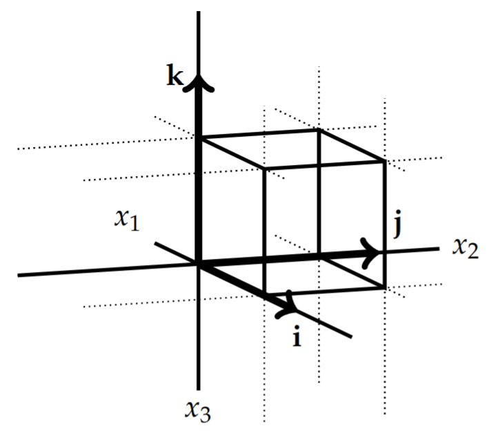
In the Cartesian system we can assign an orthogonal basis, $\{\mathbf{i}, \mathbf{j}, \mathbf{k}\}$. As a particle traces out a path in space, one locates its position by the coordinates $\left(x_{1}, x_{2}, x_{3}\right)$. Picking $x_{2}$ and $x_{3}$ constant, the particle lies on the curve $x_{1}=$ value of the $x_{1}$ coordinate. This line lies in the direction of the basis vector $\mathbf{i}$. We can do the same with the other coordinates and essentially map out a grid in three dimensional space as sown in Figure $\PageIndex{1}$. All of the $x_{i}-$ curves intersect at each point orthogonally and the basis vectors $\{\mathbf{i}, \mathbf{j}, \mathbf{k}\}$ lie along the grid lines and are mutually orthogonal. We would like to mimic this construction for general curvilinear coordinates. Requiring the orthogonality of the resulting basis vectors leads to orthogonal curvilinear coordinates.

Figure $\PageIndex{1}$: Plots of $x_{i}$-curves forming an orthogonal Cartesian grid.

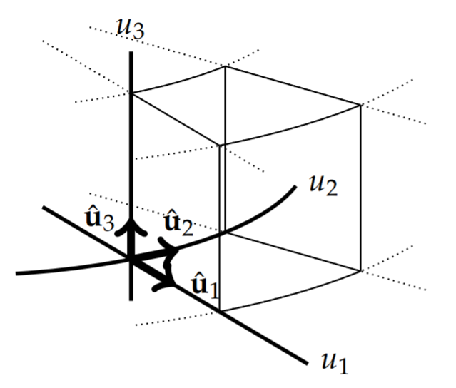
As for the Cartesian case, we consider $u_{2}$ and $u_{3}$ constant. This leads to a curve parametrized by $u_{1}: \mathbf{r}=x_{1}\left(u_{1}\right) \mathbf{i}+x_{2}\left(u_{1}\right) \mathbf{j}+x_{3}\left(u_{1}\right) \mathbf{k}$. We call this the $u_{1}$-curve. Similarly, when $u_{1}$ and $u_{3}$ are constant we obtain a $u_{2}$-curve and for $u_{1}$ and $u_{2}$ constant we obtain a $u_{3}$-curve. We will assume that these curves intersect such that each pair of curves intersect orthogonally as seen in Figure $\PageIndex{2}$. Furthermore, we will assume that the unit tangent vectors to these curves form a right handed system similar to the $\{\mathbf{i}, \mathbf{j}, \mathbf{k}\}$ systems for Cartesian coordinates. We will denote these as $\left\{\hat{\mathbf{u}}_{1}, \hat{\mathbf{u}}_{2}, \hat{\mathbf{u}}_{3}\right\}$.

Figure $\PageIndex{2}$: Plots of general $u_{i}$-curves forming an orthogonal grid.

We can determine these tangent vectors from the coordinate transformations. Consider the position vector as a function of the new coordinates,

$$\mathbf{r}\left(u_{1}, u_{2}, u_{3}\right)=x_{1}\left(u_{1}, u_{2}, u_{3}\right) \mathbf{i}+x_{2}\left(u_{1}, u_{2}, u_{3}\right) \mathbf{j}+x_{3}\left(u_{1}, u_{2}, u_{3}\right) \mathbf{k} .\nonumber$$

Then, the infinitesimal change in position is given by

$$d \mathbf{r}=\frac{\partial \mathbf{r}}{\partial u_{1}} d u_{1}+\frac{\partial \mathbf{r}}{\partial u_{2}} d u_{2}+\frac{\partial \mathbf{r}}{\partial u_{3}} d u_{3}=\sum_{i=1}^{3} \frac{\partial \mathbf{r}}{\partial u_{i}} d u_{i} \text {. }\nonumber$$

We note that the vectors $\frac{\partial \mathbf{r}}{\partial u_{i}}$ are tangent to the $u_{i}$-curves. Thus, we define the unit tangent vectors

$$\hat{\mathbf{u}}_{i}=\frac{\frac{\partial \mathbf{r}}{\partial u_{i}}}{\left|\frac{\partial \mathbf{r}}{\partial u_{i}}\right|} .\nonumber$$

Solving for the original tangent vector, we have

$$\frac{\partial \mathbf{r}}{\partial u_{i}}=h_{i} \hat{\mathbf{u}}_{i} \text {, }\nonumber$$

where

$$h_{i} \equiv\left|\frac{\partial \mathbf{r}}{\partial u_{i}}\right| .\nonumber$$

The $h_{i}$ ’s are called the scale factors for the transformation. The infinitesimal change in position in the new basis is then given by

$$d \mathbf{r}=\sum_{i=1}^{3} h_{i} u_{i} \hat{\mathbf{u}}_{i} .\nonumber$$

Note

The scale factors, $h_{i} \equiv\left|\frac{\partial \mathrm{r}}{\partial u_{i}}\right|$.

Example $\PageIndex{1}$

Determine the scale factors for the polar coordinate transformation.

Solution

The transformation for polar coordinates is

$$x=r \cos \theta, \quad y=r \sin \theta .\nonumber$$

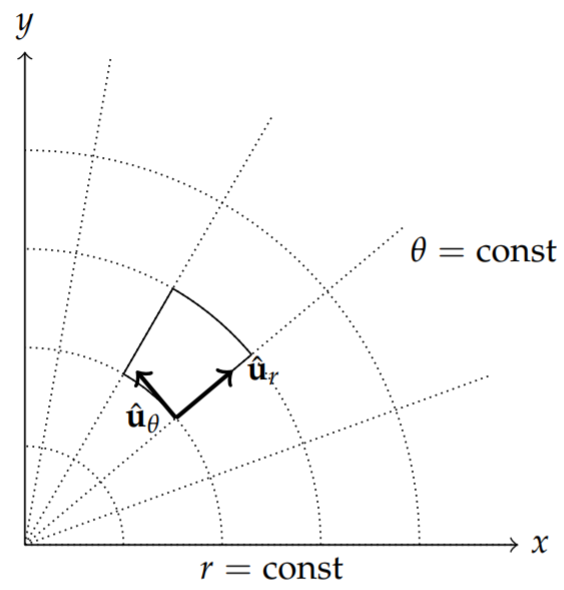
Here we note that $x_{1}=x, x_{2}=y, u_{1}=r$, and $u_{2}=\theta$. The $u_{1}$-curves are curves with $\theta=$ const. Thus, these curves are radial lines. Similarly, the $u_{2}$-curves have $r=$ const. These curves are concentric circles about the origin as shown in Figure $\PageIndex{3}$.

Figure $\PageIndex{3}$: Plots an orthogonal polar grid.

The unit vectors are easily found. We will denote them by $\hat{\mathbf{u}}_{r}$ and $\hat{\mathbf{u}}_{\theta}$. We can determine these unit vectors by first computing $\frac{\partial \mathbf{r}}{\partial u_{i}}$. Let

$$\mathbf{r}=x(r, \theta) \mathbf{i}+y(r, \theta) \mathbf{j}=r \cos \theta \mathbf{i}+r \sin \theta \mathbf{j} .\nonumber$$

Then,

$$\begin{align} &\frac{\partial \mathbf{r}}{\partial r}=\cos \theta \mathbf{i}+\sin \theta \mathbf{j}\nonumber \\ &\frac{\partial \mathbf{r}}{\partial \theta}=-r \sin \theta \mathbf{i}+r \cos \theta \mathbf{j} .\label{eq:2} \end{align}$$

The first vector already is a unit vector. So,

$$\hat{\mathbf{u}}_{r}=\cos \theta \mathbf{i}+\sin \theta \mathbf{j} .\nonumber$$

The second vector has length $r$ since $|-r \sin \theta \mathbf{i}+r \cos \theta \mathbf{j}|=r$. Dividing $\frac{\partial \mathbf{r}}{\partial \theta}$ by $r$, we have

$$\hat{\mathbf{u}}_{\theta}=-\sin \theta \mathbf{i}+\cos \theta \mathbf{j} .\nonumber$$

We can see these vectors are orthogonal $\left(\hat{\mathbf{u}}_{r} \cdot \hat{\mathbf{u}}_{\theta}=0\right)$ and form a right hand system. That they form a right hand system can be seen by either drawing the vectors, or computing the cross product,

$$\begin{align} (\cos \theta \mathbf{i}+\sin \theta \mathbf{j}) \times(-\sin \theta \mathbf{i}+\cos \theta \mathbf{j}) &=\cos ^{2} \theta \mathbf{i} \times \mathbf{j}-\sin ^{2} \theta \mathbf{j} \times \mathbf{i}\nonumber \\ &=\mathbf{k} .\label{eq:3} \end{align}$$

Since

$$\begin{aligned} &\frac{\partial \mathbf{r}}{\partial r}=\hat{\mathbf{u}}_{r}, \\ &\frac{\partial \mathbf{r}}{\partial \theta}=r \hat{\mathbf{u}}_{\theta}, \end{aligned} \nonumber$$

The scale factors are $h_{r}=1$ and $h_{\theta}=r$.

Once we know the scale factors, we have that

$$d \mathbf{r}=\sum_{i=1}^{3} h_{i} d u_{i} \hat{\mathbf{u}}_{i} .\nonumber$$

The infinitesimal arclength is then given by the Euclidean line element

$$d s^{2}=d \mathbf{r} \cdot d \mathbf{r}=\sum_{i=1}^{3} h_{i}^{2} d u_{i}^{2}\nonumber$$

when the system is orthogonal. The $h_{i}^{2}$ are referred to as the metric coefficients.

Figure $\PageIndex{4}$: Infinitesimal area in polar coordinates.

Example $\PageIndex{2}$

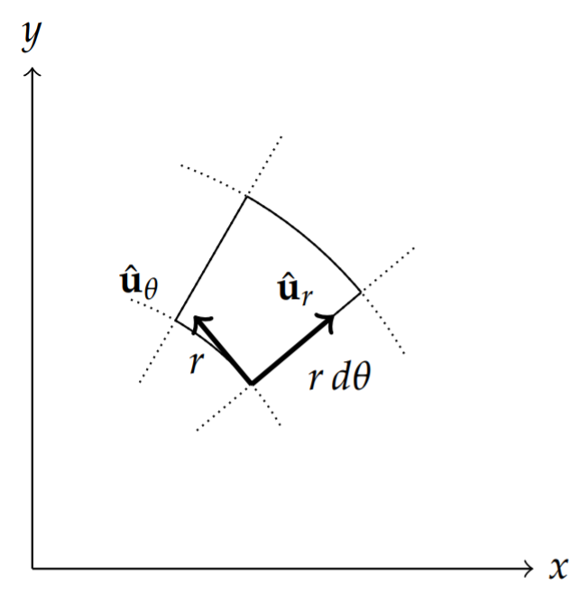
Verify that $d \mathbf{r}=d r \hat{u}_{r}+r d \theta \hat{\mathbf{u}}_{\theta}$ directly from $\mathbf{r}=r \cos \theta \mathbf{i}+r \sin \theta \mathbf{j}$ and obtain the Euclidean line element for polar coordinates.

Solution

We begin by computing

$$\begin{align} d \mathbf{r} &=d(r \cos \theta \mathbf{i}+r \sin \theta \mathbf{j})\nonumber \\ &=(\cos \theta \mathbf{i}+\sin \theta \mathbf{j}) d r+r(-\sin \theta \mathbf{i}+\cos \theta \mathbf{j}) d \theta\nonumber \\ &=d r \hat{\mathbf{u}}_{r}+r d \theta \hat{\mathbf{u}}_{\theta} .\label{eq:4} \end{align}$$

This agrees with the form $d \mathbf{r}=\sum_{i=1}^{3} h_{i} d u_{i} \hat{\mathbf{u}}_{i}$ when the scale factors for polar coordinates are inserted.

The line element is found as

$$\begin{align}ds^2&=d\mathbf{r}\cdot d\mathbf{r} \nonumber \\ &=(dr\mathbf{\hat{u}}_r+rd\theta\mathbf{\hat{u}}_\theta )\cdot (dr\mathbf{\hat{u}}_r+rd\theta\mathbf{\hat{u}}_\theta )\nonumber \\ &=dr^2+r^2d\theta ^2.\label{eq:5}\end{align}$$

This is the Euclidean line element in polar coordinates.

Also, along the $u_{i}$-curves,

$$d \mathbf{r}=h_{i} d u_{i} \hat{\mathbf{u}}_{i}, \quad \text { (no summation). }\nonumber$$

This can be seen in Figure $\PageIndex{5}$ by focusing on the $u_{1}$ curve. Along this curve, $u_{2}$ and $u_{3}$ are constant. So, $d u_{2}=0$ and $d u_{3}=0$. This leaves $d \mathbf{r}=h_{1} d u_{1} \hat{\mathbf{u}}_{1}$ along the $u_{1}$-curve. Similar expressions hold along the other two curves.

Figure $\PageIndex{5}$: Infinitesimal volume element with sides of length $h_{i} d u_{i}$.

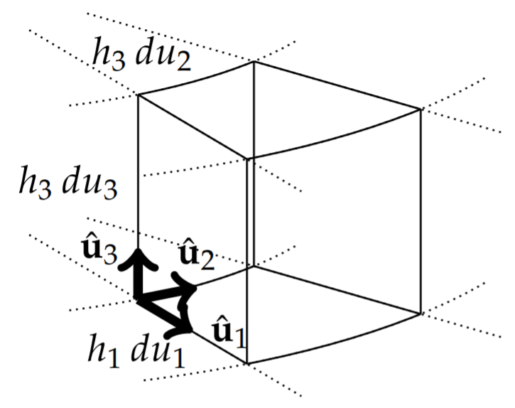
We can use this result to investigate infinitesimal volume elements for general coordinate systems as shown in Figure $\PageIndex{5}$. At a given point $\left(u_{1}, u_{2}, u_{3}\right)$ we can construct an infinitesimal parallelepiped of sides $h_{i} d u_{i}$, $i=1,2,3$. This infinitesimal parallelepiped has a volume of size

$$d V=\left|\frac{\partial \mathbf{r}}{\partial u_{1}} \cdot \frac{\partial \mathbf{r}}{\partial u_{2}} \times \frac{\partial \mathbf{r}}{\partial u_{3}}\right| d u_{1} d u_{2} d u_{3} .\nonumber$$

The triple scalar product can be computed using determinants and the resulting determinant is call the Jacobian, and is given by

$$\begin{align} J &=\left|\frac{\partial\left(x_{1}, x_{2}, x_{3}\right)}{\partial\left(u_{1}, u_{2}, u_{3}\right)}\right|\nonumber \\ &=\left|\frac{\partial \mathbf{r}}{\partial u_{1}} \cdot \frac{\partial \mathbf{r}}{\partial u_{2}} \times \frac{\partial \mathbf{r}}{\partial u_{3}}\right|\nonumber \\ &=\left|\begin{array}{ccc} \frac{\partial x_{1}}{\partial u_{1}} & \frac{\partial x_{2}}{\partial u_{1}} & \frac{\partial x_{3}}{\partial u_{1}} \\ \frac{\partial x_{1}}{\partial u_{2}} & \frac{\partial x_{2}}{\partial u_{2}} & \frac{\partial x_{3}}{\partial u_{2}} \\ \frac{\partial x_{1}}{\partial u_{3}} & \frac{\partial x_{2}}{\partial u_{3}} & \frac{\partial x_{3}}{\partial u_{3}} \end{array}\right| .\label{eq:6} \end{align}$$

Therefore, the volume element can be written as

$$d V=J d u_{1} d u_{2} d u_{3}=\left|\frac{\partial\left(x_{1}, x_{2}, x_{3}\right)}{\partial\left(u_{1}, u_{2}, u_{3}\right)}\right| d u_{1} d u_{2} d u_{3} .\nonumber$$

Example $\PageIndex{3}$

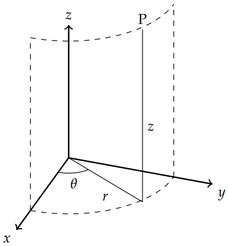
Determine the volume element for cylindrical coordinates $(r, \theta, z)$, given by

$$\begin{align} &x=r \cos \theta,\label{eq:7} \\ &y=r \sin \theta,\label{eq:8} \\ &z=z .\label{eq:9} \end{align}$$

Solution

Here, we have $\left(u_{1}, u_{2}, u_{3}\right)=(r, \theta, z)$ as displayed in Figure $\PageIndex{6}$. Then, the Jacobian is given by

$$\begin{align} J &=\mid \begin{array}{ll} \frac{\partial(x, y, z)}{\partial(r, \theta, z)} & \mid \nonumber \\ & =\left|\begin{array}{ccc} \frac{\partial x}{\partial r} & \frac{\partial y}{\partial r} & \frac{\partial z}{\partial r} \\ \frac{\partial x}{\partial \theta} & \frac{\partial y}{\partial \theta} & \frac{\partial z}{\partial \theta} \\ \frac{\partial x}{\partial z} & \frac{\partial y}{\partial z} & \frac{\partial z}{\partial z} \end{array}\right|\nonumber \\ & =\left|\begin{array}{ccc} \cos \theta & \sin \theta & 0 \\ -r \sin \theta & r \cos \theta & 0 \\ 0 & 0 & 1 \end{array}\right|\nonumber \\ & =r \end{array}\label{eq:10} \end{align}$$

Thus, the volume element is given as

$$d V=r d r d \theta d z .\nonumber$$

This result should be familiar from multivariate calculus.

Figure $\PageIndex{6}$: Cylindrical coordinate system.

Another approach is to consider the geometry of the infinitesimal volume element. The directed edge lengths are given by $d \mathbf{s}_{i}=h_{i} d u_{i} \hat{\mathbf{u}}_{i}$ as seen in Figure $\PageIndex{2}$. The infinitesimal area element of for the face in direction $\hat{\mathbf{u}}_{k}$ is found from a simple cross product,

$$d \mathbf{A}_{k}=d \mathbf{s}_{i} \times d \mathbf{s}_{j}=h_{i} h_{j} d u_{i} d u_{j} \hat{\mathbf{u}}_{i} \times \hat{\mathbf{u}}_{j} .\nonumber$$

Since these are unit vectors, the areas of the faces of the infinitesimal volumes are $d A_{k}=h_{i} h_{j} d u_{i} d u_{j}$.

The infinitesimal volume is then obtained as

$$d V=\left|d \mathbf{s}_{k} \cdot d \mathbf{A}_{k}\right|=h_{i} h_{j} h_{k} d u_{i} d u_{j} d u_{k}\left|\hat{\mathbf{u}}_{i} \cdot\left(\hat{\mathbf{u}}_{k} \times \hat{\mathbf{u}}_{j}\right)\right| .\nonumber$$

Thus, $d V=h_{1} h_{2} h_{3} d u_{1} d u_{1} d u_{3}$. Of course, this should not be a surprise since

$$J=\left|\frac{\partial \mathbf{r}}{\partial u_{1}} \cdot \frac{\partial \mathbf{r}}{\partial u_{2}} \times \frac{\partial \mathbf{r}}{\partial u_{3}}\right|=\left|h_{1} \hat{\mathbf{u}}_{1} \cdot h_{2} \hat{\mathbf{u}}_{2} \times h_{3} \hat{\mathbf{u}}_{3}\right|=h_{1} h_{2} h_{3} .\nonumber$$

Example $\PageIndex{4}$

For polar coordinates, determine the infinitesimal area element.

Solution

In an earlier example, we found the scale factors for polar coordinates as $h_{r}=1$ and $h_{\theta}=r$. Thus, $d A=h_{r} h_{\theta} d r d \theta=r d r d \theta$. Also, the last example for cylindrical coordinates will yield similar results if we already know the scales factors without having to compute the Jacobian directly. Furthermore, the area element perpendicular to the z-coordinate gives the polar coordinate system result.

Next we will derive the forms of the gradient, divergence, and curl in curvilinear coordinates using several of the identities in section ??. The results are given here for quick reference.

Note

Gradient, divergence and curl in orthogonal curvilinear coordinates.

$$\begin{align} \nabla \phi=& \sum_{i=1}^{3} \frac{\hat{u}_{i}}{h_{i}} \frac{\partial \phi}{\partial u_{i}}\nonumber \\ =& \frac{\hat{u}_{1}}{h_{1}} \frac{\partial \phi}{\partial u_{1}}+\frac{\hat{u}_{2}}{h_{2}} \frac{\partial \phi}{\partial u_{2}}+\frac{\hat{u}_{3}}{h_{3}} \frac{\partial \phi}{\partial u_{3}} \cdot\label{eq:11} \\ \nabla \cdot \mathbf{F}=& \frac{1}{h_{1} h_{2} h_{3}}\left(\frac{\partial}{\partial u_{1}}\left(h_{2} h_{3} F_{1}\right)+\frac{\partial}{\partial u_{2}}\left(h_{1} h_{3} F_{2}\right)+\frac{\partial}{\partial u_{3}}\left(h_{1} h_{2} F_{3}\right)\right)\label{eq:12} \\ \nabla \times \mathbf{F}=& \frac{1}{h_{1} h_{2} h_{3}}\left|\begin{array}{ccc} h_{1} \hat{u}_{1} & h_{2} \hat{u}_{2} & h_{3} \hat{u}_{3} \\ \frac{\partial}{\partial u_{1}} & \frac{\partial}{\partial u_{2}} & \frac{\partial}{\partial u_{3}} \\ F_{1} h_{1} & F_{2} h_{2} & F_{3} h_{3} \end{array}\right| .\label{eq:13} \\ \nabla^{2} \phi=& \frac{1}{h_{1} h_{2} h_{3}}\left(\frac{\partial}{\partial u_{1}}\left(\frac{h_{2} h_{3}}{h_{1}} \frac{\partial \phi}{\partial u_{1}}\right)+\frac{\partial}{\partial u_{2}}\left(\frac{h_{1} h_{3}}{h_{2}} \frac{\partial \phi}{\partial u_{2}}\right)\right. \\ &\left.+\frac{\partial}{\partial u_{3}}\left(\frac{h_{1} h_{2}}{h_{3}} \frac{\partial \phi}{\partial u_{3}}\right)\right) \label{eq:14} \end{align}$$

Note

Derivation of the gradient form.

We begin the derivations of these formulae by looking at the gradient, $\nabla \phi$, of the scalar function $\phi\left(u_{1}, u_{2}, u_{3}\right)$. We recall that the gradient operator appears in the differential change of a scalar function,

$$d \phi=\nabla \phi \cdot d \mathbf{r}=\sum_{i=1}^{3} \frac{\partial \phi}{\partial u_{i}} d u_{i} .\nonumber$$

Since

$$d \mathbf{r}=\sum_{i=1}^{3} h_{i} d u_{i} \hat{\mathbf{u}}_{i}\label{eq:15}$$

we also have that

$$d \phi=\nabla \phi \cdot d \mathbf{r}=\sum_{i=1}^{3}(\nabla \phi)_{i} h_{i} d u_{i} .\nonumber$$

Comparing these two expressions for $d \phi$, we determine that the components of the del operator can be written as

$$(\nabla \phi)_{i}=\frac{1}{h_{i}} \frac{\partial \phi}{\partial u_{i}}\nonumber$$

and thus the gradient is given by

$$\nabla \phi=\frac{\hat{\mathrm{u}}_{1}}{h_{1}} \frac{\partial \phi}{\partial u_{1}}+\frac{\hat{\mathrm{u}}_{2}}{h_{2}} \frac{\partial \phi}{\partial u_{2}}+\frac{\hat{\mathrm{u}}_{3}}{h_{3}} \frac{\partial \phi}{\partial u_{3}} .\label{eq:16}$$

Note

Derivation of the divergence form.

Next we compute the divergence,

$$\nabla \cdot \mathbf{F}=\sum_{i=1}^{3} \nabla \cdot\left(F_{i} \hat{\mathbf{u}}_{i}\right) .\nonumber$$

We can do this by computing the individual terms in the sum. We will compute $\nabla \cdot\left(F_{1} \hat{\mathbf{u}}_{1}\right)$.

Using Equation $\eqref{eq:16}$, we have that

$$\nabla u_{i}=\frac{\hat{\mathbf{u}}_{i}}{h_{i}} .\nonumber$$

Then

$$\nabla u_{2} \times \nabla u_{3}=\frac{\hat{\mathbf{u}}_{2} \times \hat{\mathbf{u}}_{3}}{h_{2} h_{3}}=\frac{\hat{\mathbf{u}}_{1}}{h_{2} h_{3}}\nonumber$$

Solving for $\hat{\mathbf{u}}_{1}$, gives

$$\hat{\mathbf{u}}_{1}=h_{2} h_{3} \nabla u_{2} \times \nabla u_{3} .\nonumber$$

Inserting this result into $\nabla \cdot\left(F_{1} \hat{\mathbf{u}}_{1}\right)$ and using the vector identity $2 c$ from section ??,

$$\nabla \cdot(f \mathbf{A})=f \nabla \cdot \mathbf{A}+\mathbf{A} \cdot \nabla f,\nonumber$$

we have

$$\begin{align} \nabla \cdot\left(F_{1} \hat{\mathbf{u}}_{1}\right) &=\nabla \cdot\left(F_{1} h_{2} h_{3} \nabla u_{2} \times \nabla u_{3}\right)\nonumber \\ &=\nabla\left(F_{1} h_{2} h_{3}\right) \cdot \nabla u_{2} \times \nabla u_{3}+F_{1} h_{2} h_{2} \nabla \cdot\left(\nabla u_{2} \times \nabla u_{3}\right)\label{eq:17} \end{align}$$

The second term of this result vanishes by vector identity $3 c$,

$$\nabla \cdot(\nabla f \times \nabla g)=0 .\nonumber$$

Since $\nabla u_{2} \times \nabla u_{3}=\frac{\hat{1}_{1}}{h_{2} h_{3}}$, the first term can be evaluated as

$$\nabla \cdot\left(F_{1} \hat{\mathbf{u}}_{1}\right)=\nabla\left(F_{1} h_{2} h_{3}\right) \cdot \frac{\hat{\mathbf{u}}_{1}}{h_{2} h_{3}}=\frac{1}{h_{1} h_{2} h_{3}} \frac{\partial}{\partial u_{1}}\left(F_{1} h_{2} h_{3}\right) .\nonumber$$

Similar computations can be carried out for the remaining components, leading to the sought expression for the divergence in curvilinear coordinates:

$$\nabla \cdot \mathbf{F}=\frac{1}{h_{1} h_{2} h_{3}}\left(\frac{\partial}{\partial u_{1}}\left(h_{2} h_{3} F_{1}\right)+\frac{\partial}{\partial u_{2}}\left(h_{1} h_{3} F_{2}\right)+\frac{\partial}{\partial u_{3}}\left(h_{1} h_{2} F_{3}\right)\right) .\label{eq:18}$$

Example $\PageIndex{5}$

Write the divergence operator in cylindrical coordinates.

Solution

In this case we have

$$\begin{align} \nabla \cdot \mathbf{F} &=\frac{1}{h_{r} h_{\theta} h_{z}}\left(\frac{\partial}{\partial r}\left(h_{\theta} h_{z} F_{r}\right)+\frac{\partial}{\partial \theta}\left(h_{r} h_{z} F_{\theta}\right)+\frac{\partial}{\partial \theta}\left(h_{r} h_{\theta} F_{z}\right)\right)\nonumber \\ &=\frac{1}{r}\left(\frac{\partial}{\partial r}\left(r F_{r}\right)+\frac{\partial}{\partial \theta}\left(F_{\theta}\right)+\frac{\partial}{\partial \theta}\left(r F_{z}\right)\right)\nonumber \\ &=\frac{1}{r} \frac{\partial}{\partial r}\left(r F_{r}\right)+\frac{1}{r} \frac{\partial}{\partial \theta}\left(F_{\theta}\right)+\frac{\partial}{\partial \theta}\left(F_{z}\right)\label{eq:19} \end{align}$$

We now turn to the curl operator. In this case, we need to evaluate

$$\nabla \times \mathbf{F}=\sum_{i=1}^{3} \nabla \times\left(F_{i} \hat{\mathbf{u}}_{i}\right)\nonumber$$

Again we focus on one term, $\nabla \times\left(F_{1} \hat{\mathbf{u}}_{1}\right)$. Using the vector identity $2 \mathrm{e}$,

$$\nabla \times(f \mathbf{A})=f \nabla \times \mathbf{A}-\mathbf{A} \times \nabla f,\nonumber$$

we have

$$\begin{align} \nabla \times\left(F_{1} \hat{\mathbf{u}}_{1}\right) &=\nabla \times\left(F_{1} h_{1} \nabla u_{1}\right)\nonumber \\ &=F_{1} h_{1} \nabla \times \nabla u_{1}-\nabla\left(F_{1} h_{1}\right) \times \nabla u_{1}\label{eq:20} \end{align}$$

The curl of the gradient vanishes, leaving

$$\nabla \times\left(F_{1} \hat{\mathbf{u}}_{1}\right)=\nabla\left(F_{1} h_{1}\right) \times \nabla u_{1} .\nonumber$$

Since $\nabla u_{1}=\frac{\hat{u}_{1}}{h_{1}}$, we have

$$\begin{align} \nabla \times\left(F_{1} \hat{\mathbf{u}}_{1}\right) &=\nabla\left(F_{1} h_{1}\right) \times \frac{\hat{\mathbf{u}}_{1}}{h_{1}}\nonumber \\ &=\left(\sum_{i=1}^{3} \frac{\hat{u}_{i}}{h_{i}} \frac{\partial\left(F_{1} h_{1}\right)}{\partial u_{i}}\right) \times \frac{\hat{\mathbf{u}}_{1}}{h_{1}} \nonumber \\ &=\frac{\hat{\mathbf{u}}_{2}}{h_{3} h_{1}} \frac{\partial\left(F_{1} h_{1}\right)}{\partial u_{3}}-\frac{\hat{\mathbf{u}}_{3}}{h_{1} h_{2}} \frac{\partial\left(F_{1} h_{1}\right)}{\partial u_{2}} .\label{eq:21} \end{align}$$

The other terms can be handled in a similar manner. The overall result is that

$$\begin{align} \nabla \times \mathbf{F}=& \frac{\hat{\mathbf{u}}_{1}}{h_{2} h_{3}}\left(\frac{\partial\left(h_{3} F_{3}\right)}{\partial u_{2}}-\frac{\partial\left(h_{2} F_{2}\right)}{\partial u_{3}}\right)+\frac{\hat{\mathbf{u}}_{2}}{h_{1} h_{3}}\left(\frac{\partial\left(h_{1} F_{1}\right)}{\partial u_{3}}-\frac{\partial\left(h_{3} F_{3}\right)}{\partial u_{1}}\right)\nonumber \\ &+\frac{\hat{\mathbf{u}}_{3}}{h_{1} h_{2}}\left(\frac{\partial\left(h_{2} F_{2}\right)}{\partial u_{1}}-\frac{\partial\left(h_{1} F_{1}\right)}{\partial u_{2}}\right)\label{eq:22} \end{align}$$

This can be written more compactly as

$$\nabla \times \mathbf{F}=\frac{1}{h_{1} h_{2} h_{3}}\left|\begin{array}{ccc} h_{1} \hat{\mathbf{u}}_{1} & h_{2} \hat{\mathbf{u}}_{2} & h_{3} \hat{\mathbf{u}}_{3} \\ \frac{\partial}{\partial u_{1}} & \frac{\partial}{\partial u_{2}} & \frac{\partial}{\partial u_{3}} \\ F_{1} h_{1} & F_{2} h_{2} & F_{3} h_{3} \end{array}\right|\label{eq:23}$$

Example $\PageIndex{6}$

Write the curl operator in cylindrical coordinates.

Solution

$$\begin{align} \nabla \times \mathbf{F}=& \frac{1}{r}\left|\begin{array}{ccc} \hat{\mathrm{e}}_{r} & r \hat{\mathrm{e}}_{\theta} & \hat{\mathrm{e}}_{z} \\ \frac{\partial}{\partial r} & \frac{\partial}{\partial \theta} & \frac{\partial}{\partial z} \\ F_{r} & r F_{\theta} & F_{z} \end{array}\right|\nonumber \\ =&\left(\frac{1}{r} \frac{\partial F_{z}}{\partial \theta}-\frac{\partial F_{\theta}}{\partial z}\right) \hat{\mathrm{e}}_{r}+\left(\frac{\partial F_{r}}{\partial z}-\frac{\partial F_{z}}{\partial r}\right) \hat{\mathrm{e}}_{\theta}\nonumber \\ &+\frac{1}{r}\left(\frac{\partial\left(r F_{\theta}\right)}{\partial r}-\frac{\partial F_{r}}{\partial \theta}\right) \hat{\mathrm{e}}_{z} .\label{eq:24} \end{align}$$

Finally, we turn to the Laplacian. In the next chapter we will solve higher dimensional problems in various geometric settings such as the wave equation, the heat equation, and Laplace’s equation. These all involve knowing how to write the Laplacian in different coordinate systems. Since $\nabla^{2} \phi=\nabla \cdot \nabla \phi$, we need only combine the results from Equations $\eqref{eq:16}$ and $\eqref{eq:18}$ for the gradient and the divergence in curvilinear coordinates. This is straight forward and gives

$$\begin{align} \nabla^{2} \phi=& \frac{1}{h_{1} h_{2} h_{3}}\left(\frac{\partial}{\partial u_{1}}\left(\frac{h_{2} h_{3}}{h_{1}} \frac{\partial \phi}{\partial u_{1}}\right)+\frac{\partial}{\partial u_{2}}\left(\frac{h_{1} h_{3}}{h_{2}} \frac{\partial \phi}{\partial u_{2}}\right)\right.\nonumber \\ &\left.+\frac{\partial}{\partial u_{3}}\left(\frac{h_{1} h_{2}}{h_{3}} \frac{\partial \phi}{\partial u_{3}}\right)\right) .\label{eq:25} \end{align}$$

The results of rewriting the standard differential operators in cylindrical and spherical coordinates are shown in Problems ?? and ??. In particular, the Laplacians are given as

Definition $\PageIndex{1}$: Cylindrical Coordinates

$$\label{eq:26}\nabla^2 f=\frac{1}{r}\frac{\partial}{\partial r}\left(r\frac{\partial f}{\partial r}\right)+\frac{1}{r^2}\frac{\partial^2 f}{\partial\theta^2}+\frac{\partial^2 f}{\partial z^2}.$$

Definition $\PageIndex{2}$: Spherical Coordinates

$$\label{eq:27}\nabla^2 f=\frac{1}{\rho^2}\frac{\partial}{\partial\rho}\left(\rho^2\frac{\partial f}{\partial\rho}\right)+\frac{1}{\rho^2\sin\theta}\frac{\partial}{\partial\theta}\left(\sin\theta\frac{\partial f}{\partial\theta}\right)+\frac{1}{\rho^2\sin^2\theta}\frac{\partial^2 f}{\partial\phi ^2}.$$