
6.8: Schrödinger Equation in Spherical Coordinates


- Last updated
- Sep 4, 2024
- Save as PDF

( \newcommand{\kernel}{\mathrm{null}\,}\)
Another important eigenvalue problem in physics is the Schrödinger equation. The time-dependent Schrödinger equation is given by
iℏ∂Ψ∂t=−ℏ22m∇2Ψ+VΨ.
Here Ψ(r,t) is the wave function, which determines the quantum state of a particle of mass m subject to a (time independent) potential, V(r). From Planck’s constant, h, one defines ℏ=h2π. The probability of finding the particle in an infinitesimal volume, dV, is given by |Ψ(r,t)|2dV, assuming the wave function is normalized,
∫all space |Ψ(r,t)|2dV=1
One can separate out the time dependence by assuming a special form, Ψ(r,t)=ψ(r)e−iEt/ℏ, where E is the energy of the particular stationary state solution, or product solution. Inserting this form into the time-dependent equation, one finds that ψ(r) satisfies the time-independent Schrödinger equation,
−ℏ22m∇2ψ+Vψ=Eψ.
Assuming that the potential depends only on the distance from the origin, V=V(ρ), we can further separate out the radial part of this solution using spherical coordinates. Recall that the Laplacian in spherical coordinates is given by
∇2=1ρ2∂∂ρ(ρ2∂∂ρ)+1ρ2sinθ∂∂θ(sinθ∂∂θ)+1ρ2sin2θ∂2∂ϕ2.
Then, the time-independent Schrödinger equation can be written as
−ℏ22m[1ρ2∂∂ρ(ρ2∂ψ∂ρ)+1ρ2sinθ∂∂θ(sinθ∂ψ∂θ)+1ρ2sin2θ∂2ψ∂ϕ2]=[E−V(ρ)]ψ.
Let’s continue with the separation of variables. Assuming that the wave function takes the form ψ(ρ,θ,ϕ)=R(ρ)Y(θ,ϕ), we obtain
−ℏ22m[Yρ2ddρ(ρ2dRdρ)+Rρ2sinθ∂∂θ(sinθ∂Y∂θ)+Rρ2sin2θ∂2Y∂ϕ2]=RY[E−V(ρ)]ψ.
Dividing by ψ=RY, multiplying by −2mρ2ℏ2, and rearranging, we have
1Rddρ(ρ2dRdρ)−2mρ2ℏ2[V(ρ)−E]=−1YLY,
where
L=1sinθ∂∂θ(sinθ∂∂θ)+1sin2θ∂2∂ϕ2.
We have a function of ρ equal to a function of the angular variables. So, we set each side equal to a constant. We will judiciously write the separation constant as ℓ(ℓ+1). The resulting equations are then
ddρ(ρ2dRdρ)−2mρ2ℏ2[V(ρ)−E]R=ℓ(ℓ+1)R,1sinθ∂∂θ(sinθ∂Y∂θ)+1sin2θ∂2Y∂ϕ2=−ℓ(ℓ+1)Y.
The second of these equations should look familiar from the last section. This is the equation for spherical harmonics,
Yℓm(θ,ϕ)=√2ℓ+12(ℓ−m)!(ℓ+m)!Pmℓeimϕ.
So, any further analysis of the problem depends upon the choice of potential, V(ρ), and the solution of the radial equation. For this, we turn to the determination of the wave function for an electron in orbit about a proton.
Historically, the first test of the Schrödinger equation was the determination of the energy levels in a hydrogen atom. This is modeled by an electron orbiting a proton. The potential energy is provided by the Coulomb potential,
V(ρ)=−e24πϵ0ρ.
Thus, the radial equation becomes
ddρ(ρ2dRdρ)+2mρ2ℏ2[e24πϵ0ρ+E]R=ℓ(ℓ+1)R.
Solution
Before looking for solutions, we need to simplify the equation by absorbing some of the constants. One way to do this is to make an appropriate change of variables. Let ρ= ar. Then, by the Chain Rule we have
ddρ=drdρddr=1addr.
Under this transformation, the radial equation becomes
ddr(r2dudr)+2ma2r2ℏ2[e24πϵ0ar+E]u=ℓ(ℓ+1)u,
where u(r)=R(ρ). Expanding the second term,
2ma2r2ℏ2[e24πϵ0ar+E]u=[mae22πϵ0ℏ2r+2mEa2ℏ2r2]u,
we see that we can define
a=2πϵ0ℏ2me2ϵ=−2mEa2ℏ2=−2(2πϵ0)2ℏ2me4E.
Using these constants, the radial equation becomes
ddr(r2dudr)+ru−ℓ(ℓ+1)u=ϵr2u.
Expanding the derivative and dividing by r2,
u′′+2ru′+1ru−ℓ(ℓ+1)r2u=ϵu.
The first two terms in this differential equation came from the Laplacian. The third term came from the Coulomb potential. The fourth term can be thought to contribute to the potential and is attributed to angular momentum. Thus, ℓ is called the angular momentum quantum number. This is an eigenvalue problem for the radial eigenfunctions u(r) and energy eigenvalues ϵ.
The solutions of this equation are determined in a quantum mechanics course. In order to get a feeling for the solutions, we will consider the zero angular momentum case, ℓ=0 :
u′′+2ru′+1ru=ϵu.
Even this equation is one we have not encountered in this book. Let’s see if we can find some of the solutions.
First, we consider the behavior of the solutions for large r. For large r the second and third terms on the left hand side of the equation are negligible. So, we have the approximate equation
u′′−ϵu=0.
Therefore, the solutions behave like u(r)=e±√ϵ for large r. For bounded solutions, we choose the decaying solution.
This suggests that solutions take the form u(r)=v(r)e−√er for some unknown function, v(r). Inserting this guess into Equation (???), gives an equation for v(r) :
rv′′+2(1−√ϵr)v′+(1−2√ϵ)v=0.
Next we seek a series solution to this equation. Let
v(r)=∞∑k=0ckrk.
Inserting this series into Equation (???), we have
∞∑k=1[k(k−1)+2k]ckrk−1+∞∑k=1[1−2√ϵ(k+1)]ckrk=0.
We can re-index the dummy variable in each sum. Let k=m in the first sum and k=m−1 in the second sum. We then find that
∞∑k=1[m(m+1)cm+(1−2m√ϵ)cm−1]rm−1=0.
Since this has to hold for all m≥1,
cm=2m√ϵ−1m(m+1)cm−1.
Further analysis indicates that the resulting series leads to unbounded solutions unless the series terminates. This is only possible if the numerator, 2m√ϵ−1, vanishes for m=n,n=1,2…. Thus,
ϵ=14n2.
Since ϵ is related to the energy eigenvalue, E, we have
En=−me42(4πϵ0)2ℏ2n2.
Inserting the values for the constants, this gives
En=−13.6eVn2.
This is the well known set of energy levels for the hydrogen atom.
The corresponding eigenfunctions are polynomials, since the infinite series was forced to terminate. We could obtain these polynomials by iterating the recursion equation for the cm ’s. However, we will instead rewrite the radial equation (???).
Let x=2√ϵr and define y(x)=v(r). Then
ddr=2√ϵddx.
This gives
2√ϵxy′′+(2−x)2√ϵy′+(1−2√ϵ)y=0.
Rearranging, we have
xy′′+(2−x)y′+12√ϵ(1−2√ϵ)y=0.
Noting that 2√ϵ=1n, this equation becomes
xy′′+(2−x)y′+(n−1)y=0.
The resulting equation is well known. It takes the form
xy′′+(α+1−x)y′+ny=0.
Solutions of this equation are the associated Laguerre polynomials. The solutions are denoted by Lαn(x). They can be defined in terms of the Laguerre polynomials,
Ln(x)=ex(ddx)n(e−xxn).
The associated Laguerre polynomials are defined as
Lmn−m(x)=(−1)m(ddx)mLn(x).
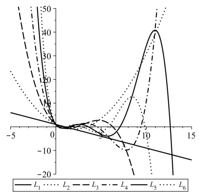
The Laguerre polynomials were first encountered in Problem 2 in Chapter 5 as an example of a classical orthogonal polynomial defined on [0,∞) with weight w(x)=e−x. Some of these polynomials are listed in Table 6.8.1 and several Laguerre polynomials are shown in Figure 6.8.1.
The associated Laguerre polynomials are named after the French mathematician Edmond Laguerre (1834-1886). In most derivation in quantum mechanicsa=a02. where a0=4πϵ0h2me2 is the Bohr radius and a0=5.2917×10⁻¹¹ m.
Comparing Equation (???) with Equation (???), we find that y(x)=L1n−1(x). In summary, we have made the following transformations:
- R(ρ)=u(r),ρ=ar.
- u(r)=v(r)e−√ϵr.
- v(r)=y(x)=L1n−1(x),x=2√ϵr.
| Lmn(x) | |
|---|---|
| L00(x) | 1 |
| L01(x) | 1−x |
| L02(x) | 12(x2−4x+2) |
| L03(x) | 16(−x3+9x2−18x+6) |
| L10(x) | 1 |
| L11(x) | 2−x |
| L12(x) | 12(x2−6x+6) |
| L13(x) | 16(−x3+3x2−36x+24) |
| L20(x) | 1 |
| L21(x) | 3−x |
| L22(x) | 12(x2−8x+12) |
| L23(x) | 112(−2x3+30x2−120x+120) |
Therefore,
R(ρ)=e−√ϵρ/aL1n−1(2√ϵρ/a).
However, we also found that 2√ϵ=1/n. So,
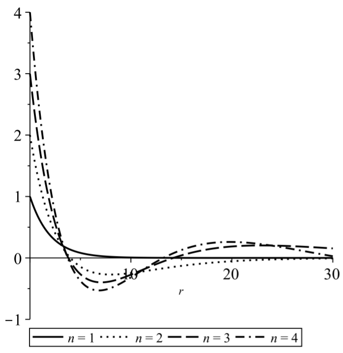
R(ρ)=e−ρ/2naL1n−1(ρ/na).
In Figure 6.8.2 we show a few of these solutions.
Find the ℓ≥0 solutions of the radial equation.
Solution
For the general case, for all ℓ≥0, we need to solve the differential equation
u′′+2ru′+1ru−ℓ(ℓ+1)r2u=ϵu.
Instead of letting u(r)=v(r)e−√ϵr, we let
u(r)=v(r)rℓe−√ϵr.
This lead to the differential equation
rv′′+2(ℓ+1−√ϵr)v′+(1−2(ℓ+1)√ϵ)v=0.
as before, we let x=2√ϵ r to obtain
xy′′+2[ℓ+1−x2]v′+[12√ϵ−ℓ(ℓ+1)]v=0.
Noting that 2√ϵ=1/n, we have
xy′′+2[2(ℓ+1)−x]v′+(n−ℓ(ℓ+1))v=0
We see that this is once again in the form of the associate Laguerre equation and the solutions are
y(x)=L2ℓ+1n−ℓ−1(x).
So, the solution to the radial equation for the hydrogen atom is given by
R(ρ)=rℓe−√ϵrL2ℓ+1n−ℓ−1(2√ϵr)=(ρ2na)ℓe−ρ/2naL2ℓ+1n−ℓ−1(ρna).
Interpretations of these solutions will be left for your quantum mechanics course.