6: Stable and Unstable Manifolds of Equilibria
- Page ID
- 24165

\( \newcommand{\vecs}[1]{\overset { \scriptstyle \rightharpoonup} {\mathbf{#1}} } \)
\( \newcommand{\vecd}[1]{\overset{-\!-\!\rightharpoonup}{\vphantom{a}\smash {#1}}} \)
\( \newcommand{\dsum}{\displaystyle\sum\limits} \)
\( \newcommand{\dint}{\displaystyle\int\limits} \)
\( \newcommand{\dlim}{\displaystyle\lim\limits} \)
\( \newcommand{\id}{\mathrm{id}}\) \( \newcommand{\Span}{\mathrm{span}}\)
( \newcommand{\kernel}{\mathrm{null}\,}\) \( \newcommand{\range}{\mathrm{range}\,}\)
\( \newcommand{\RealPart}{\mathrm{Re}}\) \( \newcommand{\ImaginaryPart}{\mathrm{Im}}\)
\( \newcommand{\Argument}{\mathrm{Arg}}\) \( \newcommand{\norm}[1]{\| #1 \|}\)
\( \newcommand{\inner}[2]{\langle #1, #2 \rangle}\)
\( \newcommand{\Span}{\mathrm{span}}\)
\( \newcommand{\id}{\mathrm{id}}\)
\( \newcommand{\Span}{\mathrm{span}}\)
\( \newcommand{\kernel}{\mathrm{null}\,}\)
\( \newcommand{\range}{\mathrm{range}\,}\)
\( \newcommand{\RealPart}{\mathrm{Re}}\)
\( \newcommand{\ImaginaryPart}{\mathrm{Im}}\)
\( \newcommand{\Argument}{\mathrm{Arg}}\)
\( \newcommand{\norm}[1]{\| #1 \|}\)
\( \newcommand{\inner}[2]{\langle #1, #2 \rangle}\)
\( \newcommand{\Span}{\mathrm{span}}\) \( \newcommand{\AA}{\unicode[.8,0]{x212B}}\)
\( \newcommand{\vectorA}[1]{\vec{#1}} % arrow\)
\( \newcommand{\vectorAt}[1]{\vec{\text{#1}}} % arrow\)
\( \newcommand{\vectorB}[1]{\overset { \scriptstyle \rightharpoonup} {\mathbf{#1}} } \)
\( \newcommand{\vectorC}[1]{\textbf{#1}} \)
\( \newcommand{\vectorD}[1]{\overrightarrow{#1}} \)
\( \newcommand{\vectorDt}[1]{\overrightarrow{\text{#1}}} \)
\( \newcommand{\vectE}[1]{\overset{-\!-\!\rightharpoonup}{\vphantom{a}\smash{\mathbf {#1}}}} \)
\( \newcommand{\vecs}[1]{\overset { \scriptstyle \rightharpoonup} {\mathbf{#1}} } \)
\(\newcommand{\longvect}{\overrightarrow}\)
\( \newcommand{\vecd}[1]{\overset{-\!-\!\rightharpoonup}{\vphantom{a}\smash {#1}}} \)
\(\newcommand{\avec}{\mathbf a}\) \(\newcommand{\bvec}{\mathbf b}\) \(\newcommand{\cvec}{\mathbf c}\) \(\newcommand{\dvec}{\mathbf d}\) \(\newcommand{\dtil}{\widetilde{\mathbf d}}\) \(\newcommand{\evec}{\mathbf e}\) \(\newcommand{\fvec}{\mathbf f}\) \(\newcommand{\nvec}{\mathbf n}\) \(\newcommand{\pvec}{\mathbf p}\) \(\newcommand{\qvec}{\mathbf q}\) \(\newcommand{\svec}{\mathbf s}\) \(\newcommand{\tvec}{\mathbf t}\) \(\newcommand{\uvec}{\mathbf u}\) \(\newcommand{\vvec}{\mathbf v}\) \(\newcommand{\wvec}{\mathbf w}\) \(\newcommand{\xvec}{\mathbf x}\) \(\newcommand{\yvec}{\mathbf y}\) \(\newcommand{\zvec}{\mathbf z}\) \(\newcommand{\rvec}{\mathbf r}\) \(\newcommand{\mvec}{\mathbf m}\) \(\newcommand{\zerovec}{\mathbf 0}\) \(\newcommand{\onevec}{\mathbf 1}\) \(\newcommand{\real}{\mathbb R}\) \(\newcommand{\twovec}[2]{\left[\begin{array}{r}#1 \\ #2 \end{array}\right]}\) \(\newcommand{\ctwovec}[2]{\left[\begin{array}{c}#1 \\ #2 \end{array}\right]}\) \(\newcommand{\threevec}[3]{\left[\begin{array}{r}#1 \\ #2 \\ #3 \end{array}\right]}\) \(\newcommand{\cthreevec}[3]{\left[\begin{array}{c}#1 \\ #2 \\ #3 \end{array}\right]}\) \(\newcommand{\fourvec}[4]{\left[\begin{array}{r}#1 \\ #2 \\ #3 \\ #4 \end{array}\right]}\) \(\newcommand{\cfourvec}[4]{\left[\begin{array}{c}#1 \\ #2 \\ #3 \\ #4 \end{array}\right]}\) \(\newcommand{\fivevec}[5]{\left[\begin{array}{r}#1 \\ #2 \\ #3 \\ #4 \\ #5 \\ \end{array}\right]}\) \(\newcommand{\cfivevec}[5]{\left[\begin{array}{c}#1 \\ #2 \\ #3 \\ #4 \\ #5 \\ \end{array}\right]}\) \(\newcommand{\mattwo}[4]{\left[\begin{array}{rr}#1 \amp #2 \\ #3 \amp #4 \\ \end{array}\right]}\) \(\newcommand{\laspan}[1]{\text{Span}\{#1\}}\) \(\newcommand{\bcal}{\cal B}\) \(\newcommand{\ccal}{\cal C}\) \(\newcommand{\scal}{\cal S}\) \(\newcommand{\wcal}{\cal W}\) \(\newcommand{\ecal}{\cal E}\) \(\newcommand{\coords}[2]{\left\{#1\right\}_{#2}}\) \(\newcommand{\gray}[1]{\color{gray}{#1}}\) \(\newcommand{\lgray}[1]{\color{lightgray}{#1}}\) \(\newcommand{\rank}{\operatorname{rank}}\) \(\newcommand{\row}{\text{Row}}\) \(\newcommand{\col}{\text{Col}}\) \(\renewcommand{\row}{\text{Row}}\) \(\newcommand{\nul}{\text{Nul}}\) \(\newcommand{\var}{\text{Var}}\) \(\newcommand{\corr}{\text{corr}}\) \(\newcommand{\len}[1]{\left|#1\right|}\) \(\newcommand{\bbar}{\overline{\bvec}}\) \(\newcommand{\bhat}{\widehat{\bvec}}\) \(\newcommand{\bperp}{\bvec^\perp}\) \(\newcommand{\xhat}{\widehat{\xvec}}\) \(\newcommand{\vhat}{\widehat{\vvec}}\) \(\newcommand{\uhat}{\widehat{\uvec}}\) \(\newcommand{\what}{\widehat{\wvec}}\) \(\newcommand{\Sighat}{\widehat{\Sigma}}\) \(\newcommand{\lt}{<}\) \(\newcommand{\gt}{>}\) \(\newcommand{\amp}{&}\) \(\definecolor{fillinmathshade}{gray}{0.9}\)For hyperbolic equilibria of autonomous vector fields, the linearization captures the local behavior near the equilibria for the nonlinear vector field. We describe the results justifying this statement in the context of two dimensional autonomous systems.
We consider a \(C^r\), \(r \ge 1\) two dimensional autonomous vector field of the following form:
\(\dot{x} = f(x,y)\),
\[\dot{y} = g(x, y), (x, y) \in \mathbb{R}^2. \label{6.1}\]
Let \(\phi_{t}(\cdot)\) denote the flow generated by (6.1). Suppose \((x_{0}, y_{0})\) is a hyperbolic equilibrium point of this vector field, i.e. the two eigenvalues of the Jacobian matrix:
\(\begin{pmatrix} {\frac{\partial f}{\partial x}(x_{0},y_{0})}&{\frac{\partial f}{\partial y}(x_{0},y_{0})}\\ {\frac{\partial g}{\partial x}(x_{0},y_{0})}&{\frac{\partial g}{\partial y}(x_{0},y_{0})} \end{pmatrix}\)
- \((x_{0}, y_{0})\) is a source for the linearized vector field,
- \((x_{0}, y_{0})\) is a sink for the linearized vector field,
- \((x_{0}, y_{0})\) is a saddle for the linearized vector field.
We consider each case individually.
- In this case \((x_{0}, y_{0})\) is a source for (6.1). More precisely, there exists a neighborhood U of \((x_{0}, y_{0})\) such that for any \(p \in U\), \(\phi_{t}(p)\) leaves U as t increases.
- In this case \((x_{0}, y_{0})\) is a sink for (6.1). More precisely, there exists a neighborhood S of \((x_{0}, y_{0})\) such that for any \(p \in S\), \(\phi_{t}(p)\) approaches \((x_{0}, y_{0})\) at an exponential rate as t increases. In this case \((x_{0}, y_{0})\) is an example of an attracting set and its basin of attraction is given by:
\(B \equiv \bigcup_{t \le 0} \phi_{t}(S).\)
- For the case of hyperbolic saddle points, the saddle point structure is still retained near the equilibrium point for nonlinear systems. We now explain precisely what this means. In order to do this we will need to examine (6.1) more closely. In particular, we will need to transform (6.1) to a coordinate system that "localizes" the behavior near the equilibrium point and specifically displays the structure of the linear part. We have already done this several times in examining the behavior near specific solutions, so we will not repeat those details.
Transforming locally near \((x_{0}, y_{0})\) in this manner, we can express (6.1) in the following form:
\[\begin{pmatrix} {\dot{\zeta}}\\ {\dot{\eta}} \end{pmatrix} = \begin{pmatrix} {-\alpha}&{0}\\ {0}&{\beta} \end{pmatrix} \begin{pmatrix} {\zeta}\\ {\eta} \end{pmatrix}+ \begin{pmatrix} {u(\zeta, \eta)}\\ {v(\zeta, \eta)} \end{pmatrix}, \alpha, \beta > 0, (\zeta, \eta) \in \mathbb{R}^2, \label{6.2}\]
where the Jacobian at the origin,
\[\begin{pmatrix} {-\alpha}&{0}\\ {0}&{\beta} \end{pmatrix}, \label{6.3}\]
reflects the hyperbolic nature of the equilibrium point. The linearization of (6.1) about the origin is given by:
\[\begin{pmatrix} {\dot{\zeta}}\\ {\dot{\eta}} \end{pmatrix} = \begin{pmatrix} {-\alpha}&{0}\\ {0}&{\beta} \end{pmatrix} \begin{pmatrix} {\zeta}\\ {\eta} \end{pmatrix}, \label{6.4}\]
It is easy to see for the linearized system that
\[E^s = {(\zeta, \eta)|\eta = 0}, \label{6.5}\]
is the invariant stable subspace and
\[E^u = {(\zeta, \eta)|\zeta = 0}, \label{6.6}\]
is the invariant unstable subspace.
We now state how this saddle point structure is inherited by the nonlinear system by stating the results of the stable and unstable manifold theorem for hyperbolic equilibria for two dimensional nonautonomous vector fields.
First, we consider two intervals of the coordinate axes containing the origin as follows:
\[I_{\zeta} \equiv {-\epsilon < \zeta < \epsilon}, \label{6.7}\]
and
\[I_{\eta} \equiv {-\epsilon < \eta < \epsilon}, \label{6.8}\]
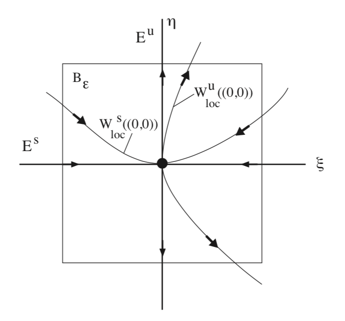
for some small \(\epsilon > 0\). A neighborhood of the origin is constructed by taking the cartesian product of these two intervals:
\[B_{\epsilon} \equiv \{(\zeta, \eta) \in \mathbb{R}^2|(\zeta, \eta) \in I_{\zeta} \times I_{\eta}\}, \label{6.9}\]
and it is illustrated in Fig. 6.1. The stable and unstable manifold theorem for hyperbolic equilibrium points of autonomous vector fields states the following.
There exists a \(C^r\) curve, given by the graph of a function of the \(\zeta\) variables:
\[\eta = S(\zeta), \zeta \in I_{\zeta}, \label{6.10}\]
This curve has three important properties.
It passes through the origin, i.e. S(0) = 0.
It is tangent to \(E^s\) at the origin, i.e., \(\frac{dS}{d\zeta} (0) = 0\).
It is locally invariant in the sense that any trajectory starting on the curve approaches the origin at an exponential rate as \(t \rightarrow \infty\), and it leaves \(B_{\epsilon}\) as \(t \rightarrow -\infty\).
Moreover, the curve satisfying these three properties is unique. For these reasons, this curve is referred to as the local stable manifold of the origin, and it is denoted by:
\[W_{loc}^{s}((0, 0)) = \{(\zeta, \eta) \in B_{\epsilon}|\eta = S(\zeta)\}. \label{6.11}\]
Similarly, there exists another \(C^{r}\) curve, given by the graph of a function of the \(\eta\) variables:
\[\zeta = U(\eta), \eta \in I_{\eta}, \label{6.12}\]
This curve has three important properties.
It passes through the origin, i.e. U(0) = 0.
It is tangent to \(E^u\) at the origin, i.e., \(\frac{dU}{d\eta} (0) = 0\).
It is locally invariant in the sense that any trajectory starting on the curve approaches the origin at an exponential rate as \(t \rightarrow -\infty\), and it leaves \(B_{\epsilon}\) as \(t \rightarrow \infty\).
For these reasons, this curve is referred to as the local unstable manifold of the origin, and it is denoted by:
\[W_{loc}^{u}((0, 0)) = \{(\zeta, \eta) \in B_{\epsilon}|\zeta = S(\zeta)\}. \label{6.13}\]
The curve satisfying these three properties is unique.
These local stable and unstable manifolds are the "seeds" for the global stable and unstable manifolds that are defined as follows:
\[W^{s} ((0, 0)) \equiv \bigcup_{t \le 0} \phi_{t}(W_{loc}^{s}((0, 0))), \label{6.14}\]
and
\[W^{u} ((0, 0)) \equiv \bigcup_{t \ge 0} \phi_{t}(W_{loc}^{u}((0, 0))), \label{6.15}\]
Now we will consider a series of examples showing how these ideas are used.
Example \(\PageIndex{13}\)
We consider the following autonomous, nonlinear vector field on the plane:
\(\dot{x} = x\),
\[\dot{y} = y + x^2, (x, y) \in \mathbb{R}^2. \label{6.16}\]
This vector field has an equilibrium point at the origin, (x, y) = (0, 0). The Jacobian of the vector field evaluated at the origin is given by:
\[\begin{pmatrix} {1}&{0}\\ {0}&{-1} \end{pmatrix}. \label{6.17}\]
From this calculation we can conclude that the origin is a hyperbolic saddle point. Moreover, the x-axis is the unstable subspace for the linearized vector field and the y axis is the stable subspace for the linearized vector field.
Next we consider the nonlinear vector field (6.16). By inspection, we see that the y axis (i.e. x = 0) is the global stable manifold for the origin. We next consider the unstable manifold. Dividing the second equation by the first equation in (6.16) gives:
\[\frac{\dot{y}}{\dot{x}} = \frac{dy}{dx} = -\frac{y}{x} + x. \label{6.18}\]
This is a linear nonautonomous equation. A solution of this equation passing through the origin is given by:
\[y = \frac{x^2}{3}, \label{6.19}\]
It is also tangent to the unstable subspace at the origin. It is the global unstable manifold.
We examine this statement further. It is easy to compute the flow generated by (6.16). The x-component can be solved and substituted into the y component to yield a first order linear nonautonomous equation. Hence, the flow generated by (6.16) is given by:
\(x(t, x_{0}) = x_{0}e^t\),
\[y(t, t_{0}) = (y_{0}-\frac{x_{0}^2}{3})e^{-t}+\frac{x_{0}^2}{3}e^{2t}, \label{6.20}\]
The global unstable manifold of the origin is the set of initial conditions having the property that the trajectories through these initial conditions approach the origin at an exponential rate as \(t \rightarrow -\infty\). On examining the two components of (6.20), we see that the x component approaches zero as \(t \rightarrow -\infty\) for any choice of \(x_{0}\). However, the y component will only approach zero as \(t \rightarrow -\infty\) if \(y_{0}\) and \(x_{0}\) are chosen such that
\[y_{0} = \frac{x_{0}^2}{3}, \label{6.21}\]
Hence (6.21) is the global unstable manifold of the origin.
Example \(\PageIndex{14}\)
Consider the following nonlinear autonomous vector field on the plane:
\(\dot{x} = x-x^3\),
\[\dot{y} = -y, (x, y) \in \mathbb{R}^2. \label{6.22}\]
Note that the x and y components evolve independently.
The equilibrium points and the Jacobians associated with their linearizations are given as follows:
\[(x, y) = (0, 0); \begin{pmatrix} {1}&{0}\\ {0}&{-1} \end{pmatrix}; saddle \label{6.23}\]
\[(x, y) = (\pm 1, 0); \begin{pmatrix} {-2}&{0}\\ {0}&{-1} \end{pmatrix}; sinks \label{6.24}\]
We now compute the global stable and unstable manifolds of these equilibria. We begin with the saddle point at the origin.
\(W^{s} ((0, 0)) = \{(x, y)|x = 0\}\)
\[W^{u} ((0, 0)) = \{(x, y)|-1 < x < 1, y = 0\} \label{6.25}\]
For the sinks the global stable manifold is synonomous with the basin of attraction for the sink.
\[(1, 0): W^{s} ((1, 0)) = \{(x, y)|x > 0\} \label{6.26}\]
\[(-1, 0): W^{s} ((-1, 0)) = \{(x, y)|x < 0\} \label{6.27}\]
Example \(\PageIndex{15}\)
In this example we consider the following nonlinear autonomous vector field on the plane:
\(\dot{x} = -x\),
\[\dot{y} = y^{2}(1-y^{2}), (x, y) \in \mathbb{R}^2. \label{6.28}\]
Note that the x and y components evolve independently.
The equilibrium points and the Jacobians associated with their linearizations are given as follows:
\[(x, y) = (0, 0), (0, \pm 1) \label{6.29}\]
\[(x, y) = (0, 0); \begin{pmatrix} {-1}&{0}\\ {0}&{0} \end{pmatrix}; not hyperbolic \label{6.30}\]
\[(x, y) = (0, 1); \begin{pmatrix} {-1}&{0}\\ {0}&{-2} \end{pmatrix}; sink \label{6.31}\]
\[(x, y) = (0, -1); \begin{pmatrix} {-1}&{0}\\ {0}&{2} \end{pmatrix}; saddle \label{6.32}\]
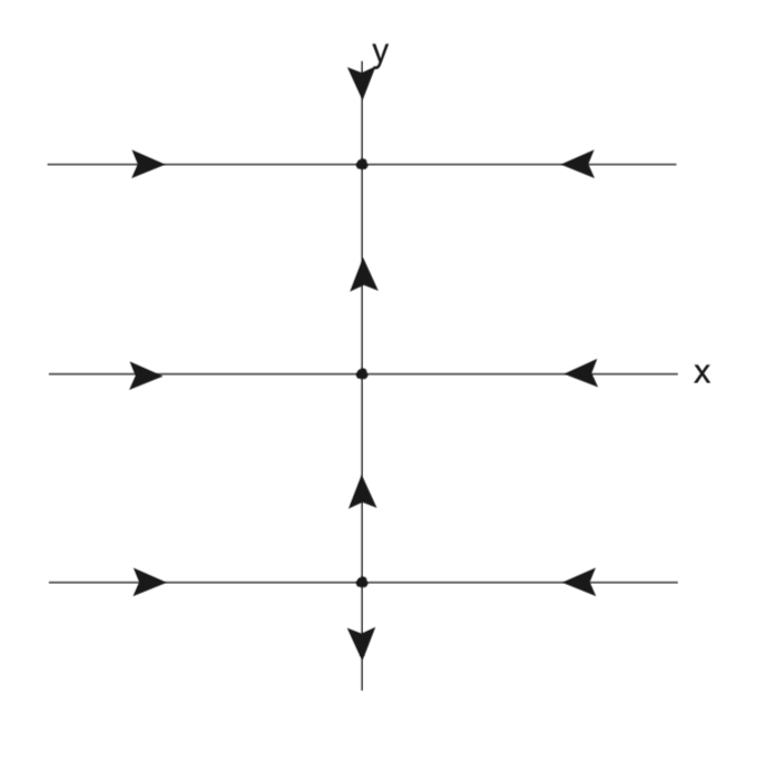
We now compute the global invariant manifold structure for each of the equilibria, beginning with (0, 0).
\(W^{s} ((0, 0)) = \{(x, y)|y = 0\}\)
\[W^{u} ((0, 0)) = \{(x, y)|-1 < y < 1, x = 0\} \label{6.33}\]
The x-axis is clearly the global stable manifold for this equilibrium point. The segment on the y-axis between \(-1\) and 1 is invariant, but it does not correspond to a hyperbolic direction. It is referred to as the center manifold of the origin, and we will learn much more about invariant manifolds associated with nonhyperbolic directions later.
The equilibrium point (0, 1) is a sink. Its global stable manifold (basin of attraction) is given by:
\[W^{s} ((0, 1)) = \{(x, y)|y > 0\} \label{6.34}\]
The equilibrium point \((0, -1)\) is a saddle point with global stable and unstable manifolds given by:
\(W^{s} ((0, -1)) = \{(x, y)|y = -1\}\)
\[W^{u} ((0, -1)) = \{(x, y)|-\infty < y < 0, x = 0\} \label{6.35}\]
Example \(\PageIndex{16}\)
In this example we consider the following nonlinear autonomous vector field on the plane:
\(\dot{x} = y\),
\[\dot{y} = x-x^{3}-\delta y, (x, y) \in \mathbb{R}^2, \delta > 0, \label{6.36}\]
where \(\delta > 0\) is to be viewed as a parameter. The equilibrium points are given by:
\[(x, y) = (0, 0), (\pm 1, 0). \label{6.37}\]
We want to classify the linearized stability of the equilibria. The Jacobian of the vector field is given by:
\[A = \begin{pmatrix} {0}&{1}\\ {1-3x^2}&{-\delta} \end{pmatrix}, \label{6.38}\]
and the eigenvalues of the Jacobian are:
\[\lambda_{\pm} = -\frac{\delta}{2} \pm \frac{1}{2}\sqrt{\delta^2+4-12x^2}. \label{6.39}\]
We evaluate this expression for the eigenvalues at each of the equilibria to determine their linearized stability.
\[(0, 0); \lambda_{\pm} = -\frac{\delta}{2} \pm \frac{1}{2}\sqrt{\delta^2+4} \label{6.40}\]
Note that
\(\delta^2+4 > \delta^2\)
therefore the eigenvalues are always real and of opposite sign. This implies that (0, 0) is a saddle.
\[(\pm 1, 0); \lambda_{\pm} = -\frac{\delta}{2} \pm \frac{1}{2}\sqrt{\delta^2-8} \label{6.41}\]
First, note that
\(\delta^2-8 < \delta^2\).
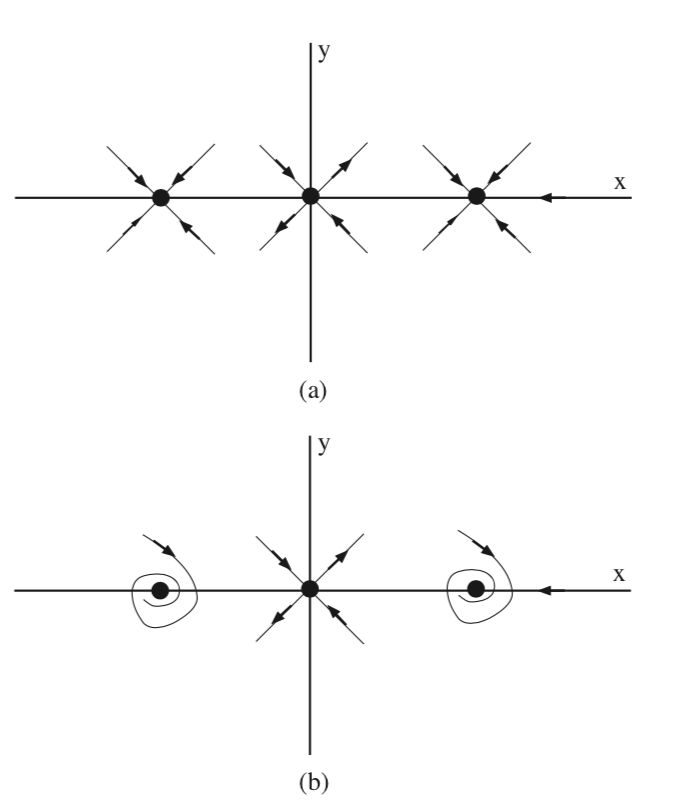
This implies that these two fixed points are always sinks. However, there are two subcases.
\(\delta^2-8 < 0\): The eigenvalues have a nonzero imaginary part.
\(\delta^2-8 > 0\): The eigenvalues are purely real.
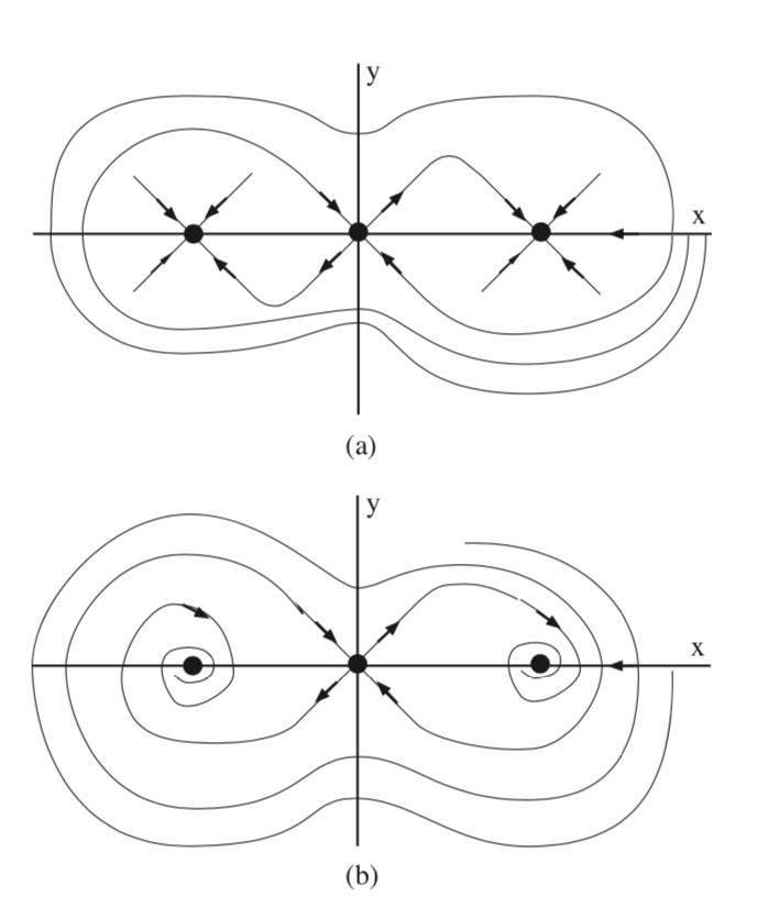
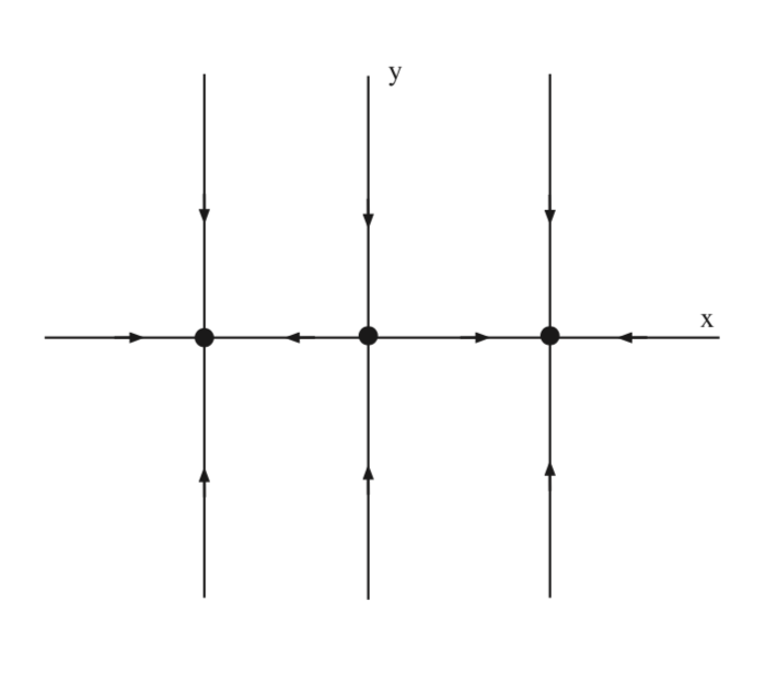
In fig. 6.4 we sketch the local invariant manifold structure for these two cases.
In fig. 6.5 we sketch the global invariant manifold structure for the two cases. In the coming lectures we will learn how we can justify this figure. However, note the role that the stable manifold of the saddle plays in defining the basins of attractions of the two sinks.