2.4: Vector Solutions to Linear Systems

Learning Objectives

• T/F: The equation \(A\vec{x}=\vec{b}\) is just another way of writing a system of linear equations.
• T/F: In solving \(A\vec{x}=\vec{0}\), if there are 3 free variables, then the solution will be “pulled apart” into 3 vectors.
• T/F: A homogeneous system of linear equations is one in which all of the coefficients are 0.
• Whether or not the equation \(A\vec{x}=\vec{b}\) has a solution depends on an intrinsic property of _____.

The first chapter of this text was spent finding solutions to systems of linear equations. We have spent the first two sections of this chapter learning operations that can be performed with matrices. One may have wondered “Are the ideas of the first chapter related to what we have been doing recently?” The answer is yes, these ideas are related. This section begins to show that relationship.

We have often hearkened back to previous algebra experience to help understand matrix algebra concepts. We do that again here. Consider the equation \(ax=b\), where \(a=3\) and \(b=6\). If we asked one to “solve for \(x\),” what exactly would we be asking? We would want to find a number, which we call \(x\), where \(a\) times \(x\) gives \(b\); in this case, it is a number, when multiplied by 3, returns 6.

Now we consider matrix algebra expressions. We’ll eventually consider solving equations like \(AX=B\), where we know what the matrices \(A\) and \(B\) are and we want to find the matrix \(X\). For now, we’ll only consider equations of the type \(A\vec{x}=\vec{b}\), where we know the matrix \(A\) and the vector \(\vec{b}\). We will want to find what vector \(\vec{x}\) satisfies this equation; we want to “solve for \(\vec{x}\).”

To help understand what this is asking, we’ll consider an example. Let

\[A=\left[\begin{array}{ccc}{1}&{1}&{1}\\{1}&{-1}&{2}\\{2}&{0}&{1}\end{array}\right],\quad\vec{b}=\left[\begin{array}{c}{2}\\{-3}\\{1}\end{array}\right]\quad\text{and}\quad\vec{x}=\left[\begin{array}{c}{x_{1}}\\{x_{2}}\\{x_{3}}\end{array}\right]. \nonumber \]

(We don’t know what \(\vec{x}\) is, so we have to represent it’s entries with the variables \(x_1\), \(x_2\) and \(x_3\).) Let’s “solve for \(\vec{x}\),” given the equation \(A\vec{x}=\vec{b}\).

We can multiply out the left hand side of this equation. We find that

\[A\vec{x}=\left[\begin{array}{c}{x_{1}+x_{2}+x_{3}}\\{x_{1}-x_{2}+2x_{3}}\\{2x_{1}+x_{3}}\end{array}\right]. \nonumber \]

Be sure to note that the product is just a vector; it has just one column.

Since \(A\vec{x}\) is equal to \(\vec{b}\), we have

\[\left[\begin{array}{c}{x_{1}+x_{2}+x_{3}}\\{x_{1}-x_{2}+2x_{3}}\\{2x_{1}+x_{3}}\end{array}\right]=\left[\begin{array}{c}{2}\\{-3}\\{1}\end{array}\right]. \nonumber \]

Knowing that two vectors are equal only when their corresponding entries are equal, we know \[\begin{align}\begin{aligned} x_1+x_2+x_3&=2\\x_1-x_2+2x_3&=-3\\2x_1+x_3&=1.\end{aligned}\end{align} \nonumber \]

This should look familiar; it is a system of linear equations! Given the matrix-vector equation \(A\vec{x}=\vec{b}\), we can recognize \(A\) as the coefficient matrix from a linear system and \(\vec{b}\) as the vector of the constants from the linear system. To solve a matrix–vector equation (and the corresponding linear system), we simply augment the matrix \(A\) with the vector \(\vec{b}\), put this matrix into reduced row echelon form, and interpret the results.

We convert the above linear system into an augmented matrix and find the reduced row echelon form:

\[\left[\begin{array}{cccc}{1}&{1}&{1}&{2}\\{1}&{-1}&{2}&{-3}\\{2}&{0}&{1}&{1}\end{array}\right]\quad\vec{\text{rref}}\quad\left[\begin{array}{cccc}{1}&{0}&{0}&{1}\\{0}&{1}&{0}&{2}\\{0}&{0}&{1}&{-1}\end{array}\right]. \nonumber \]

This tells us that \(x_1=1\), \(x_2=2\) and \(x_3 = -1\), so

\[\vec{x}=\left[\begin{array}{c}{1}\\{2}\\{-1}\end{array}\right]. \nonumber \]

We should check our work; multiply out \(A\vec{x}\) and verify that we indeed get \(\vec{b}\):

\[\left[\begin{array}{ccc}{1}&{1}&{1}\\{1}&{-1}&{2}\\{2}&{0}&{1}\end{array}\right]\:\left[\begin{array}{c}{1}\\{2}\\{-1}\end{array}\right]\quad\text{does equal}\quad\left[\begin{array}{c}{2}\\{-3}\\{1}\end{array}\right]. \nonumber \]

We should practice.

Example \(\PageIndex{1}\)

Solve the equation \(A\vec{x}=\vec{b}\) for \(\vec{x}\) where

\[A=\left[\begin{array}{ccc}{1}&{2}&{3}\\{-1}&{2}&{1}\\{1}&{1}&{0}\end{array}\right]\quad\text{and}\quad\left[\begin{array}{c}{5}\\{-1}\\{2}\end{array}\right]. \nonumber \]

Solution

The solution is rather straightforward, even though we did a lot of work before to find the answer. Form the augmented matrix \([A\:\:\vec{b}]\) and interpret its reduced row echelon form.

\[\left[\begin{array}{cccc}{1}&{2}&{3}&{5}\\{-1}&{2}&{1}&{-1}\\{1}&{1}&{0}&{2}\end{array}\right]\quad\vec{\text{rref}}\quad\left[\begin{array}{cccc}{1}&{0}&{0}&{2}\\{0}&{1}&{0}&{0}\\{0}&{0}&{1}&{1}\end{array}\right] \nonumber \]

In previous sections we were fine stating that the result as \[x_1=2, \quad x_2=0,\quad x_3=1, \nonumber \] but we were asked to find \(\vec{x}\); therefore, we state the solution as \[\vec{x}=\left[\begin{array}{c}{2}\\{0}\\{1}\end{array}\right]. \nonumber \]

This probably seems all well and good. While asking one to solve the equation \(A\vec{x}=\vec{b}\) for \(\vec{x}\) seems like a new problem, in reality it is just asking that we solve a system of linear equations. Our variables \(x_1\), etc., appear not individually but as the entries of our vector \(\vec{x}\). We are simply writing an old problem in a new way.

In line with this new way of writing the problem, we have a new way of writing the solution. Instead of listing, individually, the values of the unknowns, we simply list them as the elements of our vector \(\vec{x}\).

These are important ideas, so we state the basic principle once more: solving the equation \(A\vec{x}=\vec{b}\) for \(\vec{x}\) is the same thing as solving a linear system of equations. Equivalently, any system of linear equations can be written in the form \(A\vec{x}=\vec{b}\) for some matrix \(A\) and vector \(\vec{b}\).

Since these ideas are equivalent, we’ll refer to \(A\vec{x}=\vec{b}\) both as a matrix–vector equation and as a system of linear equations: they are the same thing.

We’ve seen two examples illustrating this idea so far, and in both cases the linear system had exactly one solution. We know from Theorem 1.4.1 that any linear system has either one solution, infinite solutions, or no solution. So how does our new method of writing a solution work with infinite solutions and no solutions?

Certainly, if \(A\vec{x}=\vec{b}\) has no solution, we simply say that the linear system has no solution. There isn’t anything special to write. So the only other option to consider is the case where we have infinite solutions. We’ll learn how to handle these situations through examples.

Example \(\PageIndex{2}\)

Solve the linear system \(A\vec{x}=\vec{0}\) for \(\vec{x}\) and write the solution in vector form, where

\[A=\left[\begin{array}{cc}{1}&{2}\\{2}&{4}\end{array}\right]\quad\text{and}\quad\vec{0}=\left[\begin{array}{c}{0}\\{0}\end{array}\right]. \nonumber \]

Solution

Note

We didn’t really need to specify that \[\vec{0}=\left[\begin{array}{c}{0}\\{0}\end{array}\right], \nonumber \] but we did just to eliminate any uncertainty.

To solve this system, put the augmented matrix into reduced row echelon form, which we do below.

\[\left[\begin{array}{ccc}{1}&{2}&{0}\\{2}&{4}&{0}\end{array}\right]\quad\vec{\text{rref}}\quad\left[\begin{array}{ccc}{1}&{2}&{0}\\{0}&{0}&{0}\end{array}\right] \nonumber \]

We interpret the reduced row echelon form of this matrix to write the solution as

\[\begin{align}\begin{aligned} x_1 &= -2x_2\\x_2 &\text{ is free.}\end{aligned}\end{align} \nonumber \]

We are not done; we need to write the solution in vector form, for our solution is the vector \(\vec{x}\). Recall that

\[\vec{x}=\left[\begin{array}{c}{x_{1}}\\{x_{2}}\end{array}\right]. \nonumber \]

From above we know that \(x_1 = -2x_2\), so we replace the \(x_1\) in \(\vec{x}\) with \(-2x_2\). This gives our solution as

\[\vec{x}=\left[\begin{array}{c}{-2x_{2}}\\{x_{2}}\end{array}\right]. \nonumber \]

Now we pull the \(x_2\) out of the vector (it is just a scalar) and write \(\vec{x}\) as

\[\vec{x}=x_{2}\left[\begin{array}{c}{-2}\\{1}\end{array}\right]. \nonumber \]

For reasons that will become more clear later, set

\[\vec{v}=\left[\begin{array}{c}{-2}\\{1}\end{array}\right]. \nonumber \]

Thus our solution can be written as

\[\vec{x}=x_{2}\vec{v}. \nonumber \]

Recall that since our system was consistent and had a free variable, we have infinite solutions. This form of the solution highlights this fact; pick any value for \(x_2\) and we get a different solution.

For instance, by setting \(x_2 = -1\), \(0\), and \(5\), we get the solutions

\[\vec{x}=\left[\begin{array}{c}{2}\\{-1}\end{array}\right],\quad\left[\begin{array}{c}{0}\\{0}\end{array}\right],\quad\text{and}\quad\left[\begin{array}{c}{-10}\\{5}\end{array}\right], \nonumber \]

respectively.

We should check our work; multiply each of the above vectors by \(A\) to see if we indeed get \(\vec{0}\).

We have officially solved this problem; we have found the solution to \(A\vec{x}=\vec{0}\) and written it properly. One final thing we will do here is graph the solution, using our skills learned in the previous section.

Our solution is

\[\vec{x}=x_{2}\left[\begin{array}{c}{-2}\\{1}\end{array}\right]. \nonumber \]

This means that any scalar multiply of the vector \(\vec{v}=\left[\begin{array}{c}{-2}\\{1}\end{array}\right]\) is a solution; we know how to sketch the scalar multiples of \(\vec{v}\). This is done in Figure \(\PageIndex{1}\).

Figure \(\PageIndex{1}\): The solution, as a line, to \(A\vec{x}=\vec{0}\) in Example \(\PageIndex{2}\).

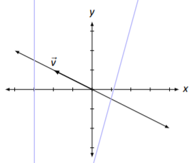
Here vector \(\vec{v}\) is drawn as well as the line that goes through the origin in the direction of \(\vec{v}\). Any vector along this line is a solution. So in some sense, we can say that the solution to \(A\vec{x}=\vec{0}\) is a line.

Let’s practice this again.

Example \(\PageIndex{3}\)

Solve the linear system \(A\vec{x}=\vec{0}\) and write the solution in vector form, where

\[A=\left[\begin{array}{cc}{2}&{-3}\\{-2}&{3}\end{array}\right]. \nonumber \]

Solution

Again, to solve this problem, we form the proper augmented matrix and we put it into reduced row echelon form, which we do below.

\[\left[\begin{array}{ccc}{2}&{-3}&{0}\\{-2}&{3}&{0}\end{array}\right]\quad\vec{\text{rref}}\quad\left[\begin{array}{ccc}{1}&{-3/2}&{0}\\{0}&{0}&{0}\end{array}\right] \nonumber \]

We interpret the reduced row echelon form of this matrix to find that \[\begin{align}\begin{aligned} x_1 &= 3/2x_2 \\ x_2 &\text{ is free.} \end{aligned}\end{align} \nonumber \]

As before,

\[\vec{x}=\left[\begin{array}{c}{x_{1}}\\{x_{2}}\end{array}\right]. \nonumber \]

Since \(x_1 = 3/2x_2\), we replace \(x_1\) in \(\vec{x}\) with \(3/2x_2\):

\[\vec{x}=\left[\begin{array}{c}{3/2x_{2}}\\{x_{2}}\end{array}\right]. \nonumber \]

Now we pull out the \(x_2\) and write the solution as

\[\vec{x}=x_{2}\left[\begin{array}{c}{3/2}\\{1}\end{array}\right]. \nonumber \]

As before, let’s set

\[\vec{v}=\left[\begin{array}{c}{3/2}\\{1}\end{array}\right] \nonumber \]

so we can write our solution as

\[\vec{x}=x_{2}\vec{v}. \nonumber \]

Again, we have infinite solutions; any choice of \(x_2\) gives us one of these solutions. For instance, picking \(x_2=2\) gives the solution

\[\vec{x}=\left[\begin{array}{c}{3}\\{2}\end{array}\right]. \nonumber \]

(This is a particularly nice solution, since there are no fractions\(\ldots\))

As in the previous example, our solutions are multiples of a vector, and hence we can graph this, as done in Figure \(\PageIndex{2}\).

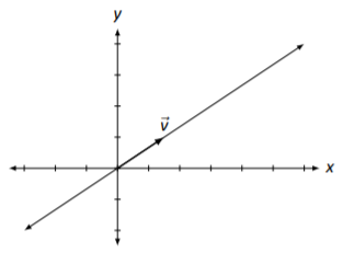
Figure \(\PageIndex{2}\): The solution, as a line, to \(A\vec{x}=\vec{0}\) in Example \(\PageIndex{3}\).

Let’s practice some more; this time, we won’t solve a system of the form \(A\vec{x}=\vec{0}\), but instead \(A\vec{x}=\vec{b}\), for some vector \(\vec{b}\).

Example \(\PageIndex{4}\)

Solve the linear system \(A\vec{x}=\vec{b}\), where

\[A=\left[\begin{array}{cc}{1}&{2}\\{2}&{4}\end{array}\right]\quad\text{and}\quad\vec{b}=\left[\begin{array}{c}{3}\\{6}\end{array}\right]. \nonumber \]

Solution

Note

This is the same matrix \(A\) that we used in Example \(\PageIndex{2}\). This will be important later.

Our methodology is the same as before; we form the augmented matrix and put it into reduced row echelon form.

\[\left[\begin{array}{ccc}{1}&{2}&{3}\\{4}&{5}&{6}\end{array}\right]\quad\vec{\text{rref}}\quad\left[\begin{array}{ccc}{1}&{2}&{3}\\{0}&{0}&{0}\end{array}\right] \nonumber \]

Interpreting this reduced row echelon form, we find that \[\begin{align}\begin{aligned} x_1 &= 3-2x_2\\ x_2 &\text{ is free.} \end{aligned}\end{align} \nonumber \] Again,

\[\vec{x}=\left[\begin{array}{c}{x_{1}}\\{x_{2}}\end{array}\right], \nonumber \]

and we replace \(x_1\) with \(3-2x_2\), giving

\[\vec{x}=\left[\begin{array}{c}{3-2x_{2}}\\{x_{2}}\end{array}\right]. \nonumber \]

This solution is different than what we’ve seen in the past two examples; we can’t simply pull out a \(x_2\) since there is a 3 in the first entry. Using the properties of matrix addition, we can “pull apart” this vector and write it as the sum of two vectors: one which contains only constants, and one that contains only “\(x_2\) stuff.” We do this below.

\[\begin{align}\begin{aligned}\vec{x}&=\left[\begin{array}{c}{3-2x_{2}}\\{x_{2}}\end{array}\right] \\ &=\left[\begin{array}{c}{3}\\{0}\end{array}\right]+\left[\begin{array}{c}{-2x_{2}}\\{x_{2}}\end{array}\right] \\ &=\left[\begin{array}{c}{3}\\{0}\end{array}\right]+x_{2}\left[\begin{array}{c}{-2}\\{1}\end{array}\right].\end{aligned}\end{align} \nonumber \]

Once again, let’s give names to the different component vectors of this solution (we are getting near the explanation of why we are doing this). Let

\[\vec{x_{p}}=\left[\begin{array}{c}{3}\\{0}\end{array}\right]\quad\text{and}\quad\vec{v}=\left[\begin{array}{c}{-2}\\{1}\end{array}\right]. \nonumber \]

We can then write our solution in the form

\[\vec{x}=\vec{x_{p}}+x_{2}\vec{v}. \nonumber \]

We still have infinite solutions; by picking a value for \(x_2\) we get one of these solutions. For instance, by letting \(x_2= -1\), \(0\), or \(2\), we get the solutions

\[\left[\begin{array}{c}{5}\\{-1}\end{array}\right],\quad\left[\begin{array}{c}{3}\\{0}\end{array}\right]\quad\text{and}\quad\left[\begin{array}{c}{-1}\\{2}\end{array}\right]. \nonumber \]

We have officially solved the problem; we have solved the equation \(A\vec{x}=\vec{b}\) for \(\vec{x}\) and have written the solution in vector form. As an additional visual aid, we will graph this solution.

Each vector in the solution can be written as the sum of two vectors: \(\vec{x_{p}}\) and a multiple of \(\vec{v}\). In Figure \(\PageIndex{3}\), \(\vec{x_{p}}\) is graphed and \(\vec{v}\) is graphed with its origin starting at the tip of \(\vec{x_{p}}\). Finally, a line is drawn in the direction of \(\vec{v}\) from the tip of \(\vec{x_{p}}\); any vector pointing to any point on this line is a solution to \(A\vec{x}=\vec{b}\).

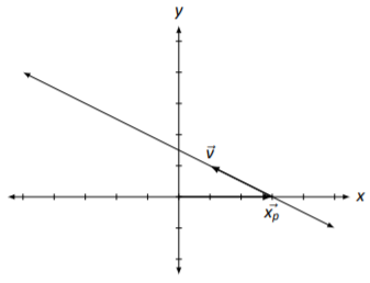
Figure \(\PageIndex{3}\): The solution, as a line, to \(A\vec{x}=\vec{b}\) in Example \(\PageIndex{4}\).

The previous examples illustrate some important concepts. One is that we can “see” the solution to a system of linear equations in a new way. Before, when we had infinite solutions, we knew we could arbitrarily pick values for our free variables and get different solutions. We knew this to be true, and we even practiced it, but the result was not very “tangible.” Now, we can view our solution as a vector; by picking different values for our free variables, we see this as multiplying certain important vectors by a scalar which gives a different solution.

Another important concept that these examples demonstrate comes from the fact that Examples \(\PageIndex{2}\) and \(\PageIndex{4}\) were only “slightly different” and hence had only “slightly different” answers. Both solutions had

\[x_{2}\left[\begin{array}{c}{-2}\\{1}\end{array}\right] \nonumber \]

in them; in Example \(\PageIndex{4}\) the solution also had another vector added to this. Was this coincidence, or is there a definite pattern here?

Of course there is a pattern! Now \(\ldots\) what exactly is it? First, we define a term.

Definition: Homogenous Linear System of Equations

A system of linear equations is homogeneous if the constants in each equation are zero.

Note: a homogeneous system of equations can be written in vector form as \(A\vec{x}=\vec{0}\).

The term homogeneous comes from two Greek words; homo meaning “same” and genus meaning “type.” A homogeneous system of equations is a system in which each equation is of the same type – all constants are 0. Notice that the system of equations in Examples \(\PageIndex{2}\) and \(\PageIndex{4}\) are homogeneous.

Note that \(A\vec{0}=\vec{0}\); that is, if we set \(\vec{x}=\vec{0}\), we have a solution to a homogeneous set of equations. This fact is important; the zero vector is always a solution to a homogeneous linear system. Therefore a homogeneous system is always consistent; we need only to determine whether we have exactly one solution (just \(\vec{0}\)) or infinite solutions. This idea is important so we give it it’s own box.

Key Idea \(\PageIndex{1}\): Homogeneous Systems and Consistency

All homogeneous linear systems are consistent.

How do we determine if we have exactly one or infinite solutions? Recall Key Idea 1.4.1: if the solution has any free variables, then it will have infinite solutions. How can we tell if the system has free variables? Form the augmented matrix \([A\:\:\vec{0}]\), put it into reduced row echelon form, and interpret the result.

It may seem that we’ve brought up a new question, “When does \(A\vec{x}=\vec{0}\) have exactly one or infinite solutions?” only to answer with “Look at the reduced row echelon form of \(A\) and interpret the results, just as always.” Why bring up a new question if the answer is an old one?

While the new question has an old solution, it does lead to a great idea. Let’s refresh our memory; earlier we solved two linear systems,

\[A\vec{x}=\vec{0}\quad\text{and}\quad A\vec{x}=\vec{b} \nonumber \]

where

\[A=\left[\begin{array}{cc}{1}&{2}\\{2}&{4}\end{array}\right]\quad\text{and}\quad\vec{b}=\left[\begin{array}{c}{3}\\{6}\end{array}\right]. \nonumber \]

The solution to the first system of equations, \(A\vec{x}=\vec{0}\), is

\[\vec{x}=x_{2}\left[\begin{array}{c}{-2}\\{1}\end{array}\right] \nonumber \]

and the solution to the second set of equations, \(A\vec{x}=\vec{b}\), is

\[\vec{x}=\left[\begin{array}{c}{3}\\{0}\end{array}\right]+x_{2}\left[\begin{array}{c}{-2}\\{1}\end{array}\right], \nonumber \]

for all values of \(x_2\).

Recalling our notation used earlier, set

\[\vec{x_{p}}=\left[\begin{array}{c}{3}\\{0}\end{array}\right]\quad\text{and let}\quad\vec{v}=\left[\begin{array}{c}{-2}\\{1}\end{array}\right]. \nonumber \]

Thus our solution to the linear system \(A\vec{x}=\vec{b}\) is

\[\vec{x}=\vec{x_{p}}+x_{2}\vec{v}. \nonumber \]

Let us see how exactly this solution works; let’s see why \(A\vec{x}\) equals \(\vec{b}\). Multiply \(A\vec{x}\):

\[\begin{align}\begin{aligned}A\vec{x}&=A(\vec{x_{p}}+x_{2}\vec{v}) \\ &=A\vec{x_{p}}+A(x_{2}\vec{v}) \\ &=A\vec{x_{p}}+x_{2}(A\vec{v}) \\ &=A\vec{x_{p}}+x_{2}\vec{0} \\ &=A\vec{x_{p}}+\vec{0} \\ &=A\vec{x_{p}} \\ &=\vec{b}\end{aligned}\end{align} \nonumber \]

We know that the last line is true, that \(A\vec{x_{p}}=\vec{b}\), since we know that \(\vec{x}\) was a solution to \(A\vec{x}=\vec{b}\). The whole point is that \(\vec{x_{p}}\) itself is a solution to \(A\vec{x}=\vec{b}\), and we could find more solutions by adding vectors “that go to zero” when multiplied by \(A\). (The subscript \(p\) of “\(\vec{x_{p}}\)” is used to denote that this vector is a “particular” solution.)

Stated in a different way, let’s say that we know two things: that \(A\vec{x_{p}}=\vec{b}\) and \(A\vec{v}=\vec{0}\). What is \(A(\vec{x_{p}}+\vec{v})\)? We can multiply it out:

\[\begin{align}\begin{aligned}A(\vec{x_{p}}+\vec{v})&=A\vec{x_{p}}+A\vec{v} \\ &=\vec{b}+\vec{0} \\ &=\vec{b}\end{aligned}\end{align} \nonumber \]

and see that \(A(\vec{x_{p}}+\vec{v})\) also equals \(\vec{b}\).

So we wonder: does this mean that \(A\vec{x}=\vec{b}\) will have infinite solutions? After all, if \(\vec{x_{p}}\) and \(\vec{x_{p}}+\vec{v}\) are both solutions, don’t we have infinite solutions?

No. If \(A\vec{x}=\vec{0}\) has exactly one solution, then \(\vec{v}=\vec{0}\), and \(\vec{x_{p}}=\vec{x_{p}}+\vec{v}\); we only have one solution.

So here is the culmination of all of our fun that started a few pages back. If \(\vec{v}\) is a solution to \(A\vec{x}=\vec{0}\) and \(\vec{x_{p}}\) is a solution to \(A\vec{x}=\vec{b}\), then \(\vec{x_{p}}+\vec{v}\) is also a solution to \(A\vec{x}=\vec{b}\). If \(A\vec{x}=\vec{0}\) has infinite solutions, so does \(A\vec{x}=\vec{b}\); if \(A\vec{x}=\vec{0}\) has only one solution, so does \(A\vec{x}=\vec{b}\). This culminating idea is of course important enough to be stated again.

Key Idea \(\PageIndex{2}\): Solutions of Consistent Systems

Let \(A\vec{x}=\vec{b}\) be a consistent system of linear equations.

1. If \(A\vec{x}=\vec{0}\) has exactly one solution \((\vec{x}=\vec{0})\), then \(A\vec{x}=\vec{b}\) has exactly one solution.
2. If \(A\vec{x}=\vec{0}\) has infinite solutions, then \(A\vec{x}=\vec{b}\) has infinite solutions.

A key word in the above statement is consistent. If \(A\vec{x}=\vec{b}\) is inconsistent (the linear system has no solution), then it doesn’t matter how many solutions \(A\vec{x}=\vec{0}\) has; \(A\vec{x}=\vec{b}\) has no solution.

Enough fun, enough theory. We need to practice.

Example \(\PageIndex{5}\)

Let

\[A=\left[\begin{array}{cccc}{1}&{-1}&{1}&{3}\\{4}&{2}&{4}&{6}\end{array}\right]\quad\text{and}\quad\vec{b}=\left[\begin{array}{c}{1}\\{10}\end{array}\right]. \nonumber \]

Solve the linear systems \(A\vec{x}=\vec{0}\) and \(A\vec{x}=\vec{b}\) for \(\vec{x}\), and write the solutions in vector form.

Solution

We’ll tackle \(A\vec{x}=\vec{0}\) first. We form the associated augmented matrix, put it into reduced row echelon form, and interpret the result.

\[\left[\begin{array}{ccccc}{1}&{-1}&{1}&{3}&{0}\\{4}&{2}&{4}&{6}&{0}\end{array}\right]\quad\vec{\text{rref}}\quad\left[\begin{array}{ccccc}{1}&{0}&{1}&{2}&{0}\\{0}&{1}&{0}&{-1}&{0}\end{array}\right] \nonumber \]

\[\begin{align}\begin{aligned} x_1&=-x_3-2x_4\\x_2 &= x_4\\ x_3&\text{ is free}\\x_4&\text{ is free} \end{aligned}\end{align} \nonumber \] To write our solution in vector form, we rewrite \(x_1\) and \(x_2\) in \(\vec{x}\) in terms of \(x_3\) and \(x_4\).

\[\vec{x}=\left[\begin{array}{c}{x_{1}}\\{x_{2}}\\{x_{3}}\\{x_{4}}\end{array}\right]=\left[\begin{array}{c}{-x_{3}-2x_{4}}\\{x_{4}}\\{x_{3}}\\{x_{4}}\end{array}\right] \nonumber \]

Finally, we “pull apart” this vector into two vectors, one with the “\(x_3\) stuff” and one with the “\(x_4\) stuff.”

\[\begin{align}\begin{aligned}\vec{x}&=\left[\begin{array}{c}{-x_{3}-2x_{4}}\\{x_{4}}\\{x_{3}}\\{x_{4}}\end{array}\right] \\ &=\left[\begin{array}{c}{-x_{3}}\\{0}\\{x_{3}}\\{0}\end{array}\right]+\left[\begin{array}{c}{-2x_{4}}\\{x_{4}}\\{0}\\{x_{4}}\end{array}\right] \\ &=x_{3}\left[\begin{array}{c}{-1}\\{0}\\{1}\\{0}\end{array}\right]+x_{4}\left[\begin{array}{c}{-2}\\{1}\\{0}\\{1}\end{array}\right] \\ &=x_{3}\vec{u}+x_{4}\vec{v}\end{aligned}\end{align} \nonumber \]

We use \(\vec{u}\) and \(\vec{v}\) simply to give these vectors names (and save some space).

It is easy to confirm that both \(\vec{u}\) and \(\vec{v}\) are solutions to the linear system \(A\vec{x}=\vec{0}\). (Just multiply \(A\vec{u}\) and \(A\vec{v}\) and see that both are \(\vec{0}\).) Since both are solutions to a homogeneous system of linear equations, any linear combination of \(\vec{u}\) and \(\vec{v}\) will be a solution, too.

Now let’s tackle \(A\vec{x}=\vec{b}\). Once again we put the associated augmented matrix into reduced row echelon form and interpret the results.

\[\left[\begin{array}{ccccc}{1}&{-1}&{1}&{3}&{1}\\{4}&{2}&{4}&{6}&{10}\end{array}\right]\quad\vec{\text{rref}}\quad\left[\begin{array}{ccccc}{1}&{0}&{1}&{2}&{2}\\{0}&{1}&{0}&{-1}&{1}\end{array}\right] \nonumber \]

\[\begin{align}\begin{aligned} x_1&=2-x_3-2x_4\\x_2 &= 1+x_4\\ x_3&\text{ is free}\\x_4&\text{ is free} \end{aligned}\end{align} \nonumber \]

Writing this solution in vector form gives

\[\vec{x}=\left[\begin{array}{c}{x_{1}}\\{x_{2}}\\{x_{3}}\\{x_{4}}\end{array}\right]=\left[\begin{array}{c}{2-x_{3}-2x_{4}}\\{1+x_{4}}\\{x_{3}}\\{x_{4}}\end{array}\right]. \nonumber \]

Again, we pull apart this vector, but this time we break it into three vectors: one with “\(x_3\)” stuff, one with “\(x_4\)” stuff, and one with just constants.

\[\begin{align}\begin{aligned}\vec{x}&=\left[\begin{array}{c}{2-x_{3}-2x_{4}}\\{1+x_{4}}\\{x_{3}}\\{x_{4}}\end{array}\right] \\ &=\left[\begin{array}{c}{2}\\{1}\\{0}\\{0}\end{array}\right] + \left[\begin{array}{c}{-x_{3}}\\{0}\\{x_{3}}\\{0}\end{array}\right] +\left[\begin{array}{c}{-2x_{4}}\\{x_{4}}\\{0}\\{x_{4}}\end{array}\right] \\ &=\left[\begin{array}{c}{2}\\{1}\\{0}\\{0}\end{array}\right] +x_{3}\left[\begin{array}{c}{-1}\\{0}\\{1}\\{0}\end{array}\right] + x_{4}\left[\begin{array}{c}{-2}\\{1}\\{0}\\{1}\end{array}\right] \\ &=\underbrace{\vec{x_{p}}}\quad +\quad \underbrace{x_{3}\vec{u}+x_{4}\vec{v}} \\ & \text{particular} \qquad \text{solution to} \\ &\text{solution}\qquad\:\:\text{homogenous} \\ &\qquad\qquad\:\:\:\:\text{equations }A\vec{x}=\vec{0} \end{aligned}\end{align} \nonumber \]

Note that \(A\vec{x_{p}}=\vec{b}\); by itself, \(\vec{x_{p}}\) is a solution. To get infinite solutions, we add a bunch of stuff that “goes to zero” when we multiply by \(A\); we add the solution to the homogeneous equations.

Why don’t we graph this solution as we did in the past? Before we had only two variables, meaning the solution could be graphed in 2D. Here we have four variables, meaning that our solution “lives” in 4D. You can draw this on paper, but it is very confusing.

Example \(\PageIndex{6}\)

Rewrite the linear system

\[\begin{array}{ccccccccccc}{x_{1}}&{+}&{2x_{2}}&{-}&{3x_{3}}&{+}&{2x_{4}}&{+}&{7x_{5}}&{=}&{2}\\ {3x_{1}}&{+}&{4x_{2}}&{+}&{5x_{3}}&{+}&{2x_{4}}&{+}&{3x_{5}}&{=}&{-4}\end{array} \nonumber \]

as a matrix–vector equation, solve the system using vector notation, and give the solution to the related homogeneous equations.

Solution

Rewriting the linear system in the form of \(A\vec{x}=\vec{b}\), we have that

\[A=\left[\begin{array}{ccccc}{1}&{2}&{-3}&{2}&{7}\\{3}&{4}&{5}&{2}&{3}\end{array}\right],\quad\vec{x}=\left[\begin{array}{c}{x_{1}}\\{x_{2}}\\{x_{3}}\\{x_{4}}\\{x_{5}}\end{array}\right]\quad\text{and}\quad\vec{b}=\left[\begin{array}{c}{2}\\{-4}\end{array}\right]. \nonumber \]

To solve the system, we put the associated augmented matrix into reduced row echelon form and interpret the results.

\[\left[\begin{array}{cccccc}{1}&{2}&{-3}&{2}&{7}&{2}\\{3}&{4}&{5}&{2}&{3}&{-4}\end{array}\right]\quad\vec{\text{rref}}\quad\left[\begin{array}{cccccc}{1}&{0}&{11}&{-2}&{-11}&{-8}\\{0}&{1}&{-7}&{2}&{9}&{5}\end{array}\right] \nonumber \]

\[\begin{align}\begin{aligned} x_1&=-8-11x_3+2x_4+11x_5\\ x_2&=5+7x_3-2x_4-9x_5\\ x_3&\text{ is free}\\ x_4&\text{ is free}\\ x_5&\text{ is free}\end{aligned}\end{align} \nonumber \]

We use this information to write \(\vec{x}\), again pulling it apart. Since we have three free variables and also constants, we’ll need to pull \(\vec{x}\) apart into four separate vectors.

\[\begin{align}\begin{aligned}\vec{x}&=\left[\begin{array}{c}{x_{1}}\\{x_{2}}\\{x_{3}}\\{x_{4}}\\{x_{5}}\end{array}\right] \\ &=\left[\begin{array}{c}{-8-11x_{3}+2x_{4}+11x_{5}}\\{5+7x_{3}-2x_{4}-9x_{5}}\\{x_{3}}\\{x_{4}}\\{x_{5}}\end{array}\right] \\ &=\left[\begin{array}{c}{-8}\\{5}\\{0}\\{0}\\{0}\end{array}\right]+\left[\begin{array}{c}{-11x_{3}}\\{7x_{3}}\\{x_{3}}\\{0}\\{0}\end{array}\right]+\left[\begin{array}{c}{2x_{4}}\\{-2x_{4}}\\{0}\\{x_{4}}\\{0}\end{array}\right]+\left[\begin{array}{c}{11x_{5}}\\{-9x_{5}}\\{0}\\{0}\\{x_{5}}\end{array}\right] \\ &=\left[\begin{array}{c}{-8}\\{5}\\{0}\\{0}\\{0}\end{array}\right] +x_{3}\left[\begin{array}{c}{-11}\\{7}\\{1}\\{0}\\{0}\end{array}\right]+x_{4}\left[\begin{array}{c}{2}\\{-2}\\{0}\\{1}\\{0}\end{array}\right]+x_{5}\left[\begin{array}{c}{11}\\{-9}\\{0}\\{0}\\{1}\end{array}\right] \\ &=\underbrace{\vec{x_{p}}}\quad+\quad \underbrace{x_{3}\vec{u}+x_{4}\vec{v}+x_{5}\vec{w}} \\ & \text{particular} \qquad \text{solution to homogenous} \\ &\text{solution}\qquad\quad\text{equations }A\vec{x}=\vec{0} \end{aligned}\end{align} \nonumber \]

So \(\vec{x_{p}}\) is a particular solution; \(A\vec{x_{p}}=\vec{b}\). (Multiply it out to verify that this is true.) The other vectors, \(\vec{u}\), \(\vec{v}\) and \(\vec{w}\), that are multiplied by our free variables \(x_3\), \(x_4\) and \(x_5\), are each solutions to the homogeneous equations, \(A\vec{x}=\vec{0}\). Any linear combination of these three vectors, i.e., any vector found by choosing values for \(x_3\), \(x_4\) and \(x_5\) in \(x_{3}\vec{u}+x_{4}\vec{v}+x_{5}\vec{w}\) is a solution to \(A\vec{x}=\vec{0}\).

Example \(\PageIndex{7}\)

Let

\[A=\left[\begin{array}{cc}{1}&{2}\\{4}&{5}\end{array}\right]\quad\text{and}\quad\vec{b}=\left[\begin{array}{c}{3}\\{6}\end{array}\right]. \nonumber \]

Find the solutions to \(A\vec{x}=\vec{b}\) and \(A\vec{x}=\vec{0}\).

Solution

We go through the familiar work of finding the reduced row echelon form of the appropriate augmented matrix and interpreting the solution.

\[\left[\begin{array}{ccc}{1}&{2}&{3}\\{4}&{5}&{6}\end{array}\right]\quad\vec{\text{rref}}\quad\left[\begin{array}{ccc}{1}&{0}&{-1}\\{0}&{1}&{2}\end{array}\right] \nonumber \]

\[\begin{align}\begin{aligned} x_1 &= -1\\x_2 &= 2\end{aligned}\end{align} \nonumber \]

Thus

\[\vec{x}=\left[\begin{array}{c}{x_{1}}\\{x_{2}}\end{array}\right]=\left[\begin{array}{c}{-1}\\{2}\end{array}\right]. \nonumber \]

This may strike us as a bit odd; we are used to having lots of different vectors in the solution. However, in this case, the linear system \(A\vec{x}=\vec{b}\) has exactly one solution, and we’ve found it. What is the solution to \(A\vec{x}=\vec{0}\)? Since we’ve only found one solution to \(A\vec{x}=\vec{b}\), we can conclude from Key Idea \(\PageIndex{2}\) the related homogeneous equations \(A\vec{x}=\vec{0}\) have only one solution, namely \(\vec{x}=\vec{0}\). We can write our solution vector \(\vec{x}\) in a form similar to our previous examples to highlight this:

\[\begin{align}\begin{aligned}\vec{x}&=\left[\begin{array}{c}{-1}\\{2}\end{array}\right] \\ &=\left[\begin{array}{c}{-1}\\{2}\end{array}\right] +\left[\begin{array}{c}{0}\\{0}\end{array}\right] \\ &=\underbrace{\vec{x_{p}}}\quad +\quad\underbrace{\vec{0}} \\ &\text{particular}\qquad\text{solution to} \\ &\text{solution}\qquad A\vec{x}=\vec{0}\end{aligned}\end{align} \nonumber \]

Example \(\PageIndex{8}\)

Let

\[A=\left[\begin{array}{cc}{1}&{1}\\{2}&{2}\end{array}\right]\quad\text{and}\quad\vec{b}=\left[\begin{array}{c}{1}\\{1}\end{array}\right]. \nonumber \]

Find the solutions to \(A\vec{x}=\vec{b}\) and \(A\vec{x}=\vec{0}\).

Solution

To solve \(A\vec{x}=\vec{b}\), we put the appropriate augmented matrix into reduced row echelon form and interpret the results.

\[\left[\begin{array}{ccc}{1}&{1}&{1}\\{2}&{2}&{1}\end{array}\right]\quad\vec{\text{rref}}\quad\left[\begin{array}{ccc}{1}&{1}&{0}\\{0}&{0}&{1}\end{array}\right] \nonumber \]

We immediately have a problem; we see that the second row tells us that \(0x_1+0x_2 = 1\), the sign that our system does not have a solution. Thus \(A\vec{x}=\vec{b}\) has no solution. Of course, this does not mean that \(A\vec{x}=\vec{0}\) has no solution; it always has a solution.

To find the solution to \(A\vec{x}=\vec{0}\), we interpret the reduced row echelon from of the appropriate augmented matrix.

\[\left[\begin{array}{ccc}{1}&{1}&{0}\\{2}&{2}&{0}\end{array}\right]\quad\vec{\text{rref}}\quad\left[\begin{array}{ccc}{1}&{1}&{0}\\{0}&{0}&{0}\end{array}\right] \nonumber \]

\[\begin{align}\begin{aligned} x_1 &=-x_2 \\ x_2 &\text{ is free} \end{aligned}\end{align} \nonumber \]

Thus

\[\begin{align}\begin{aligned}\vec{x}&=\left[\begin{array}{c}{x_{1}}\\{x_{2}}\end{array}\right] \\ &=\left[\begin{array}{c}{-x_{2}}\\{x_{2}}\end{array}\right] \\ &=x_{2}\left[\begin{array}{c}{-1}\\{1}\end{array}\right] \\ &=x_{2}\vec{u}.\end{aligned}\end{align} \nonumber \]

We have no solution to \(A\vec{x}=\vec{b}\), but infinite solutions to \(A\vec{x}=\vec{0}\).

The previous example may seem to violate the principle of Key Idea \(\PageIndex{2}\). After all, it seems that having infinite solutions to \(A\vec{x}=\vec{0}\) should imply infinite solutions to \(A\vec{x}=\vec{b}\). However, we remind ourselves of the key word in the idea that we observed before: consistent. If \(A\vec{x}=\vec{b}\) is consistent and \(A\vec{x}=\vec{0}\) has infinite solutions, then so will \(A\vec{x}=\vec{b}\). But if \(A\vec{x}=\vec{b}\) is not consistent, it does not matter how many solutions \(A\vec{x}=\vec{0}\) has; \(A\vec{x}=\vec{b}\) is still inconsistent.
This whole section is highlighting a very important concept that we won’t fully understand until after two sections, but we get a glimpse of it here. When solving any system of linear equations (which we can write as \(A\vec{x}=\vec{b}\)), whether we have exactly one solution, infinite solutions, or no solution depends on an intrinsic property of \(A\). We’ll find out what that property is soon; in the next section we solve a problem we introduced at the beginning of this section, how to solve matrix equations \(AX=B\).