Overview
- Page ID
- 70180
The Subject of This Textbook
Before starting with the content of the text, we first ask the basic question: what is linear algebra?
- Linear: having to do with lines, planes, etc.
- Algebra: solving equations involving unknowns.
The name of the textbook highlights an important theme: the synthesis between algebra and geometry. It will be very important to us to understand systems of linear equations both algebraically (writing equations for their solutions) and geometrically (drawing pictures and visualizing).
The term “algebra” was coined by the \(9\)th century mathematician Abu Ja’far Muhammad ibn Musa al-Khwarizmi. It comes from the Arabic word al-jebr, meaning reunion of broken parts.
At the simplest level, solving a system of linear equations is not very hard. You probably learned in high school how to solve a system like
\[\left\{\begin{array}{rrrrrrr}{x}&{+}&{3y}&{-}&{z}&{=}&{4} \\ 2x&-&y&+&3z&=&17 \\ {}&{}&{y}&{-}&{4z}&{=}&{-3.}\end{array}\right. \nonumber\]
However, in real life one usually has to be more clever.
- Engineers need to solve many, many equations in many, many variables. Here is a tiny example:
\[\left\{\begin{array}{rrrrrrrrrrrrr}3x_1 & +&4x_2 &+&10x_3&+&19x_4&-&2x_5&-&3x_6&=&141 \\ 7x_1 &+&2x_2&-&13x_3&-&7x_4&+&21x_5&+&8x_6&=& 2567 \\ -x_1 &+& 9x_2 &+& \frac 32x_3 &+& x_4 &+& 14x_5& + &27x_6 &=& 26 \\ \frac 12x_1 &+& 4x_2 &+& 10x_3 &+& 11x_4 &+& 2x_5 &+& x_6 &=& -15 \end{array}\right. \nonumber\] - Often it is enough to know some information about the set of solutions, without having to solve the equations in the first place. For instance, does there exist a solution? What does the solution set look like geometrically? Is there still a solution if we change the \(26\) to a \(27\text{?}\)
- Sometimes the coefficients also contain parameters, like the eigenvalue equation
\[\left\{\begin{array}{rrrrrrr} (7-\lambda)x &+& y &+& 3z &=& 0 \\ -3x& +& (2-\lambda)y &-& 3z &=& 0 \\ -3x &-& 2y& +& (-1-\lambda)z &=& 0\end{array}\right. \nonumber\] - In data modeling, a system of equations generally does not actually have a solution. In that case, what is the best approximate solution?
Accordingly, this text is organized into three main sections.
-
Solve the matrix equation \(Ax=b\) (chapters 2–4).
- Solve systems of linear equations using matrices, row reduction, and inverses.
- Analyze systems of linear equations geometrically using the geometry of solution sets and linear transformations.
-
Solve the matrix equation \(Ax=\lambda x\) (chapters 5–6).
- Solve eigenvalue problems using the characteristic polynomial.
- Understand the geometry of matrices using similarity, eigenvalues, diagonalization, and complex numbers.
-
Approximately solve the matrix equation \(Ax=b\) (chapter 7).
- Find best-fit solutions to systems of linear equations that have no actual solution using least-squares approximations.
- Study the geometry of closest vectors and orthogonal projections.
This text is roughly half computational and half conceptual in nature. The main goal is to present a library of linear algebra tools, and more importantly, to teach a conceptual framework for understanding which tools should be applied in a given context.
If Matlab can find the answer faster than you can, then your question is just an algorithm: this is not real problem solving.
The subtle part of the subject lies in understanding what computation to ask the computer to do for you—it is far less important to know how to perform computations that a computer can do better than you anyway.
Uses of Linear Algebra in Engineering
The vast majority of undergraduates at Georgia Tech have to take a course in linear algebra. There is a reason for this:
Most engineering problems, no matter how complicated, can be reduced to linear algebra:
\[ Ax=b \quad\text{or}\quad Ax=\lambda x \quad\text{or}\quad Ax\approx b. \nonumber \]
Here we present some sample problems in science and engineering that require linear algebra to solve.
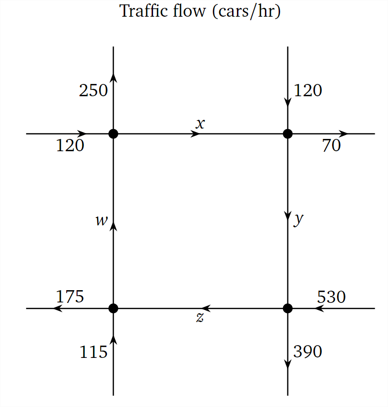
The following diagram represents traffic flow around the town square. The streets are all one way, and the numbers and arrows indicate the number of cars per hour flowing along each street, as measured by sensors underneath the roads.

Figure \(\PageIndex{1}\)
There are no sensors underneath some of the streets, so we do not know how much traffic is flowing around the square itself. What are the values of \(x,y,z,w\text{?}\) Since the number of cars entering each intersection has to equal the number of cars leaving that intersection, we obtain a system of linear equations:
\[\left\{\begin{array}{rrrrrrr} w &+& 120 &=& x &+& 250\\ x &+& 120 &=& y &+& 70\\ y &+& 530 &=& z &+& 390\\ z &+& 115 &=& w &+& 175 \end{array}\right.\nonumber\]
A certain chemical reaction (burning) takes ethane and oxygen, and produces carbon dioxide and water:
\[\underline{x}\:\text{C}_{2}\text{H}_{6}\:+\:\underline{y}\:\text{O}_{2}\:\to\:\underline{z}\:\text{CO}_{2}\:+\:\underline{w}\:\text{H}_{2}\text{O}\nonumber\]
What ratio of the molecules is needed to sustain the reaction? The following three equations come from the fact that the number of atoms of carbon, hydrogen, and oxygen on the left side has to equal the number of atoms on the right, respectively:
\[ \begin{split} 2x \amp= z \\ 6x \amp= 2w \\ 2y \amp= 2z + w\rlap. \end{split} \nonumber \]
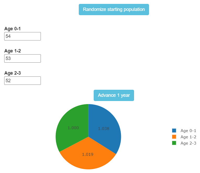
In a population of rabbits,
- half of the newborn rabbits survive their first year;
- of those, half survive their second year;
- the maximum life span is three years;
- rabbits produce 0, 6, 8 baby rabbits in their first, second, and third years, respectively.
If you know the rabbit population in 2016 (in terms of the number of first, second, and third year rabbits), then what is the population in 2017? The rules for reproduction lead to the following system of equations, where \(x,y,z\) represent the number of newborn, first-year, and second-year rabbits, respectively:
\[\left\{\begin{array}{rrrrrrr} {}&{}&6y_{2016} &+& 8z_{2016} &=& x_{2017}\\ \frac 12x_{2016} &{}&{}&{}&{}&=& y_{2017}\\ {}&{}& \frac 12y_{2016}&{}&{}& =& z_{2017}\end{array}\right. \nonumber\]
A common question is: what is the asymptotic behavior of this system? What will the rabbit population look like in 100 years? This turns out to be an eigenvalue problem.

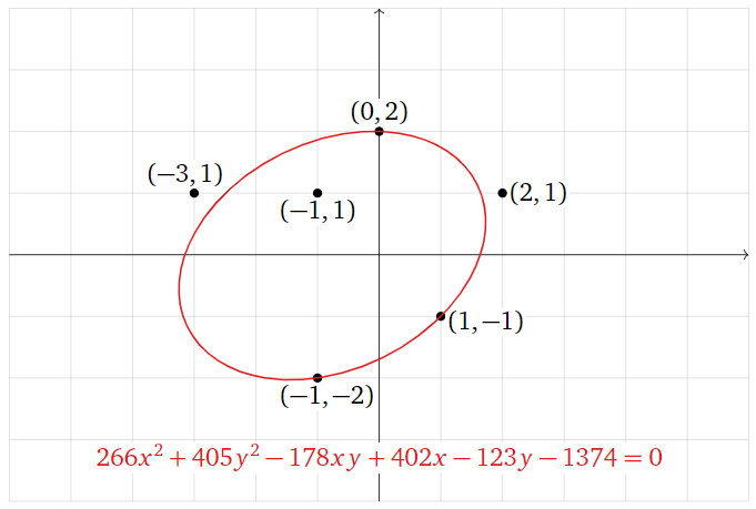
An asteroid has been observed at the following locations:
\[ (0,2),\, (2,1),\, (1,-1),\, (-1,-2),\, (-3,1),\, (-1,-1). \nonumber \]
Its orbit around the sun is elliptical; it is described by an equation of the form
\[ x^2 + By^2 + Cxy + Dx + Ey + F = 0. \nonumber \]
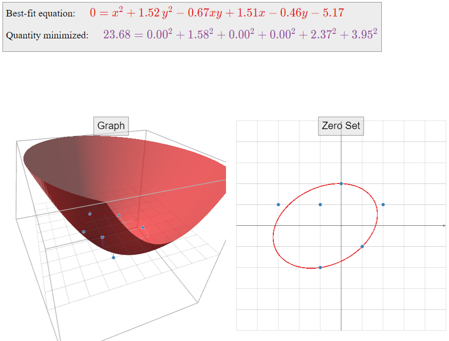
What is the most likely orbit of the asteroid, given that there was some significant error in measuring its position? Substituting the data points into the above equation yields the system
\[\begin{array}{rrrrrrrrrrrrl} (0)^2 &+& B(2)^2 &+& C(0)(2) &+& D(0) &+& E(2)&+& F&=&0 \\ (2)^2 &+& B(1)^2 &+& C(2)(1) &+& D(2) &+& E(1) &+& F&=& 0 \\ (1)^2 &+& B(-1)^2 &+& C(1)(-1) &+& D(1) &+& E(-1) &+& F&=& 0 \\ (-1)^2 &+& B(-2)^2 &+& C(-1)(-2) &+& D(-1)&+& E(-2)&+&F&=& 0 \\ (-3)^2 &+& B(1)^2 &+& C(-3)(1) &+& D(-3)&+& E(1)&+& F&=& 0 \\ (-1)^2 &+& B(-1)^2 &+& C(-1)(-1)&+& D(-1)&+& E(-1)&+&F&=&0. \end{array}\nonumber\]
There is no actual solution to this system due to measurement error, but here is the best-fitting ellipse:

Figure \(\PageIndex{3}\)
Each web page has some measure of importance, which it shares via outgoing links to other pages. This leads to zillions of equations in zillions of variables. Larry Page and Sergei Brin realized that this is a linear algebra problem at its core, and used the insight to found Google. We will discuss this example in detail in Section 5.5. The result is the so-called “25 billion dollar eigenvector.” See Section 6.6 in the full version of the book for a detailed discussion of this example.
How to Use This Textbook
There are a number of different categories of ideas that are contained in most sections. They are listed at the top of the section, under Objectives, for easy review. We classify them as follows.
- Recipes: these are algorithms that are generally straightforward (if sometimes tedious), and are usually done by computer in real life. They are nonetheless important to learn and to practice.
- Vocabulary words: forming a conceptual understanding of the subject of linear algebra means being able to communicate much more precisely than in ordinary speech. The vocabulary words have precise definitions, which must be learned and used correctly.
- Essential vocabulary words: these vocabulary words are essential in that they form the essence of the subject of linear algebra. For instance, if you do not know the definition of an eigenvector, then by definition you cannot claim to understand linear algebra.
- Theorems: these describe in a precise way how the objects of interest relate to each other. Knowing which recipe to use in a given situation generally means recognizing which vocabulary words to use to describe the situation, and understanding which theorems apply to that problem.
- Pictures: visualizing the geometry underlying the algebra means interpreting and drawing pictures of the objects involved. The pictures are meant to be a core part of the material in the text: they are not just a pretty add-on.
This textbook is exclusively targeted at Math 1553 at Georgia Tech. As such, it contains exactly the material that is taught in that class; no more, and no less: students in Math 1553 are responsible for understanding all visible content. In the online version some extra material (most examples and proofs, for instance) is hidden, in that one needs to click on a link to reveal it, like this:
Finally, we remark that there are over 140 interactive demos contained in the text, which were created to illustrate the geometry of the topic. Click the “view in a new window” link, and play around with them! You will need a modern browser. Internet Explorer is not a modern browser; try Safari, Chrome, or Firefox. Here is a demo from Section 6.4:

Feedback
Every page of the online version has a link on the bottom for providing feedback. This will take you to the GitHub Issues page for this book. It requires a Georgia Tech login to access.


