2.8: Bases as Coordinate Systems

Objectives

1. Learn to view a basis as a coordinate system on a subspace.
2. Recipes: compute the $\mathcal{B}$-coordinates of a vector, compute the usual coordinates of a vector from its $\mathcal{B}$-coordinates.
3. Picture: the $\mathcal{B}$-coordinates of a vector using its location on a nonstandard coordinate grid.
4. Vocabulary word: $\mathcal{B}$-coordinates.

In this section, we interpret a basis of a subspace $V$ as a coordinate system on $V$, and we learn how to write a vector in $V$ in that coordinate system.

Fact $\PageIndex{1}$

If $\mathcal{B}=\{v_1,\: v_2,\cdots ,v_m\}$ is a basis for a subspace $V$, then any vector $x$ in $V$ can be written as a linear combination

$$x=c_1v_1+c_2v_2+\cdots +c_mv_m\nonumber$$

in exactly one way.

Proof

Recall that to say $\mathcal{B}$ is a basis for $V$ means that $\mathcal{B}$ spans $V$ and $\mathcal{B}$ is linearly independent. Since $\mathcal{B}$ spans $V$, we can write any $x$ in $V$ as a linear combination of $v_1,\: v_2,\cdots ,v_m$. For uniqueness, suppose that we had two such expressions:

$$\begin{aligned}x&=c_1v_1+c_2v_2+\cdots +c_mv_m \\ x&=c_1'v_1+c_2'v_2+\cdots +c_m'v_m.\end{aligned}$$

Subtracting the first equation from the second yields

$$0=x-x=(c_1-c_1')v_1 +(c_2-c_2')v_2+\cdots +(c_m-c_m')v_m.\nonumber$$

Since $\mathcal{B}$ is linearly independent, the only solution to the above equation is the trivial solution: all the coefficients must be zero. It follows that $c_i−c_i'$ for all $i$, which proves that $c_1=c_1',\: c_2=c_2',\cdots ,c_m=c_m'$.

Example $\PageIndex{1}$

Consider the standard bases of $\mathbb{R}^{3}$ from Example 2.7.3 in Section 2.7.

$$e_1=\left(\begin{array}{c}1\\0\\0\end{array}\right),\quad e_2=\left(\begin{array}{c}0\\1\\0\end{array}\right),\quad e_3=\left(\begin{array}{c}0\\0\\1\end{array}\right).\nonumber$$

According to the above fact, Fact $\PageIndex{1}$, every vector in $\mathbb{R}^{3}$ can be written as a linear combination of $e_1$, $e_2$, $e_3$, with unique coefficients. For example,

$$v=\left(\begin{array}{c}\color{Red}{3}\\ \color{blue}{5} \\ \color{Green}{-2}\end{array}\right)\color{black}{=}\color{red}{3}\color{black}{\left(\begin{array}{c}1\\0\\0\end{array}\right)+}\color{blue}{5}\color{black}{\left(\begin{array}{c}0\\1\\0\end{array}\right)}\color{Green}{-2}\color{black}{\left(\begin{array}{c}0\\0\\1\end{array}\right)=}\color{Red}{3}\color{black}{e_1+}\color{blue}{5}\color{black}{e_2}\color{Green}{-2}\color{black}{e_3.}\nonumber$$

In this case, the coordinates of $v$ are exactly the coefficients of $e_1$, $e_2$, $e_3$.

What exactly are coordinates, anyway? One way to think of coordinates is that they give directions for how to get to a certain point from the origin. In the above example, the linear combination $3e_1+5e_2−2e_3$ can be thought of as the following list of instructions: start at the origin, travel $3$ units north, then travel $5$ units east, then $2$ units down.

Definition $\PageIndex{1}$: $\mathcal{B}$-Coordinate Vector

Let $\mathcal{B}=\{v_1,\: v_2,\cdots ,v_m\}$ be a basis of a subspace $V$, and let

$$x=c_1v_1+c_2v_2+\cdots+c_mv_m\nonumber$$

be a vector in $V$. The coefficients $c_1,\:c_2,\cdots,c_m$ are the coordinates of $x$ with respect to $\mathcal{B}$. The $\mathcal{B}$-coordinate vector of $x$ is the vector

$$[x]_{\mathcal{B}}=\left(\begin{array}{c}c_1 \\c_2\\ \vdots \\ c_m\end{array}\right)\quad\text{ in }\mathbb{R}^{m}.\nonumber$$

If we change the basis, then we can still give instructions for how to get to the point $(3,\:5,\:−2)$, but the instructions will be different. Say for example we take the basis

$$v_1=e_1+e_2=\left(\begin{array}{c}1\\1\\0\end{array}\right),\quad v_2=e_2=\left(\begin{array}{c}0\\1\\0\end{array}\right),\quad v_3=e_3=\left(\begin{array}{c}0\\0\\1\end{array}\right).\nonumber$$

We can write $(3,\:5,\:−2)$ in this basis as $3v_1+2v_2−2v_3$. In other words: start at the origin, travel northeast $3$ times as far as $v_1$, then $2$ units east, then $2$ units down. In this situation, we can say that “$3$ is the $v_1$-coordinate of $(3,\:5,\:−2)$, $2$ is the $v_2$-coordinate of $(3,\:5,\:−2)$, and $−2$ is the $v_3$-coordinate of $(3,\:5,\:−2)$.”

Note $\PageIndex{1}$

The above definition, Definition $\PageIndex{1}$, gives a way of using $\mathbb{R}_m$ to label the points of a subspace of dimension $m$: a point is simply labeled by its $\mathcal{B}$-coordinate vector. For instance, if we choose a basis for a plane, we can label the points of that plane with the points of $\mathbb{R}^2$.

Example $\PageIndex{2}$: A Nonstandard Coordinate System of $\mathbb{R}^2$)

Define

$$v_1=\left(\begin{array}{c}1\\1\end{array}\right),\quad v_2=\left(\begin{array}{c}1\\-1\end{array}\right),\quad\mathcal{B}=\{v_1,\:v_2\}.\nonumber$$

1. Verify that $\mathcal{B}$ is a basis for $\mathbb{R}^2$.
2. If $[w]_{\mathcal{B}}=\left(\begin{array}{c}1\\2\end{array}\right)$, then what is $w$?
3. Find the $\mathcal{B}$-coordinates of $v=\left(\begin{array}{c}5\\3\end{array}\right)$.

Solution

1. By the basis theorem in Section 2.7, Theorem 2.7.3, any two linearly independent vectors form a basis for $\mathbb{R}^2$. Clearly $v_1,\:v_2$ are not multiples of each other, so they are linearly independent.
2. To say $[w]_{\mathcal{B}}=\left(\begin{array}{c}1\\2\end{array}\right)$ means that $1$ is the $v_1$-coordinate of $w$, and that $2$ is the $v_2$-coordinate:
   $$w=v_1+2v_2=\left(\begin{array}{c}1\\1\end{array}\right)+2\left(\begin{array}{c}1\\-1\end{array}\right)=\left(\begin{array}{c}3\\-1\end{array}\right).\nonumber$$
3. We have to solve the vector equation $v=c_1v_1+c_2v_2$ in the unknowns $c_1,\: c_2$. We form an augmented matrix and row reduce:
   $$\left(\begin{array}{cc|c} 1&1&5 \\ 1&-1&3\end{array}\right)  \quad\xrightarrow{\text{RREF}}\quad\left(\begin{array}{cc|c} 1&0&4 \\ 0&1&1\end{array}\right).\nonumber$$
   We have $c_1=4$ and $c_2=1$, so $v=4v_1+v_2$ and $[v]_{\mathcal{B}}=\left(\begin{array}{c}4\\1\end{array}\right)$.

In the following picture, we indicate the coordinate system defined by $\mathcal{B}$ by drawing lines parallel to the “$v_1$-axis” and “$v_2$-axis”. Using this grid it is easy to see that the $\mathcal{B}$-coordinates of $v$ are $\left(\begin{array}{c}5\\1\end{array}\right)$, and that the $\mathcal{B}$-coordinates of $w$ are $\left(\begin{array}{c}1\\2\end{array}\right)$.

Figure $\PageIndex{1}$

This picture could be the grid of streets in Palo Alto, California. Residents of Palo Alto refer to northwest as “north” and to northeast as “east”. There is a reason for this: the old road to San Francisco is called El Camino Real, and that road runs from the southeast to the northwest in Palo Alto. So when a Palo Alto resident says “go south two blocks and east one block”, they are giving directions from the origin to the Whole Foods at $w$.

Figure $\PageIndex{2}$: A picture of the basis $\mathcal{B}=\{v_1,\: v_2\}$ of $\mathbb{R}^2$. The grid indicates the coordinate system defined by the basis $\mathcal{B}$; one set of lines measures the $v_1$-coordinate, and the other set measures the $v_2$-coordinate. Use the sliders to find the $\mathcal{B}$-coordinates of $w$.

Example $\PageIndex{3}$

Let

$$v_1=\left(\begin{array}{c}2\\-1\\1\end{array}\right)\quad v_2=\left(\begin{array}{c}1\\0\\-1\end{array}\right).\nonumber$$

These form a basis $\mathcal{B}$ for a plane $V=\text{Span}\{v_1,\: v_2\}$ in $\mathbb{R}^3$. We indicate the coordinate system defined by $\mathcal{B}$ by drawing lines parallel to the “$v_1$-axis” and “$v_2$-axis”:

Figure $\PageIndex{3}$

We can see from the picture that the $v_1$-coordinate of $\color{red}{u_1}$ is equal to $1$, as is the $v_2$-coordinate, so $[\color{red}{u_1}\color{black}{]_{\mathcal{B}}=\left(\begin{array}{c}1\\1\end{array}\right)}$. Similarly, we have

$$[\color{blue}{u_2}\color{black}{]_{\mathcal{B}}}=\left(\begin{array}{c}-1 \\ \frac{1}{2}\end{array}\right)\quad [\color{Green}{u_3}\color{black}{]_{\mathcal{B}}}=\left(\begin{array}{c}\frac{3}{2} \\ -\frac{1}{2}\end{array}\right)\quad [\color{orange}{u_4}\color{black}{]_{\mathcal{B}}}=\left(\begin{array}{c}0\\ \frac{3}{2}\end{array}\right).\nonumber$$

Figure $\PageIndex{4}$: Left: the $\mathcal{B}$-coordinates of a vector $x$. Right: the vector $x$. The violet grid on the right is a picture of the coordinate system defined by the basis $\mathcal{B}$; one set of lines measures the $v_1$-coordinate, and the other set measures the $v_2$-coordinate. Drag the heads of the vectors $x$ and $[x]_{\mathcal{B}}$ to understand the correspondence between $x$ and its $\mathcal{B}$-coordinate vector.

Example $\PageIndex{4}$: A Coordinate System on a Plane

Define

$$v_1=\left(\begin{array}{c}1\\0\\1\end{array}\right),\: v_2=\left(\begin{array}{c}1\\1\\1\end{array}\right),\quad\mathcal{B}=\{v_1,\: v_2\},\quad V=\text{Span}\{v_1,\: v_2\}.\nonumber$$

1. Verify that $\mathcal{B}$ is a basis for $V$.
2. If $[w]_{\mathcal{B}}=\left(\begin{array}{c}5\\2\end{array}\right)$, then what is $w$?
3. Find the $\mathcal{B}$-coordinates of $v=\left(\begin{array}{c}5\\3\\5\end{array}\right)$.

Solution

1. We need to verify that $\mathcal{B}$ spans $V$, and that it is linearly independent. By definition, $V$ is the span of $\mathcal{B}$; since $v_1$ and $v_2$ are not multiples of each other, they are linearly independent. This shows in particular that $V$ is a plane.
2. To say $[w]_{\mathcal{B}}=\left(\begin{array}{c}5\\2\end{array}\right)$ means that $5$ is the $v_1$-coordinate of $w$, and that $2$ is the $v_2$-coordinate:
   $$w=5v_1 +2v_2=5\left(\begin{array}{c}1\\0\\1\end{array}\right)+2\left(\begin{array}{c}1\\1\\1\end{array}\right)=\left(\begin{array}{c}7\\2\\7\end{array}\right).\nonumber$$
3. We have to solve the vector equation $v=c_1v_1+c_2v_2$ in the unknowns $c_1,\: c_2$. We form an augmented matrix and row reduce:
   $$\left(\begin{array}{cc|c} 1&1&5\\0&1&3\\1&1&5\end{array}\right) \quad\xrightarrow{\text{RREF}}\quad \left(\begin{array}{cc|c} 1&0&2\\0&1&3\\0&0&0\end{array}\right).\nonumber$$

We have $c_1=2$ and $c_2=3$, so $v=2v_1+3v_2$ and $[v]_{\mathcal{B}}=\left(\begin{array}{c}2\\3\end{array}\right)$.

Figure $\PageIndex{5}$: A picture of the plane $V$ and the basis $\mathcal{B}=\{v_1,\: v_2\}$. The violet grid is a picture of the coordinate system defined by the basis $\mathcal{B}$; one set of lines measures the $v_1$-coordinate, and the other set measures the $v_2$-coordinate. Use the sliders to find the $\mathcal{B}$-coordinates of $v$.

Example $\PageIndex{5}$: A Coordinate System on Another Plane

Define

$$v_1=\left(\begin{array}{c}2\\3\\2\end{array}\right),\quad v_2=\left(\begin{array}{c}-1\\1\\1\end{array}\right),\quad v_3=\left(\begin{array}{c}2\\8\\6\end{array}\right),\quad V=\text{Span}\{v_1,\: v_2,\: v_3\}.\nonumber$$

1. Find a basis $\mathcal{B}$ for $V$.
2. Find the $\mathcal{B}$-coordinates of $x=\left(\begin{array}{c}4\\11\\8\end{array}\right).$

Solution

1. We write $V$ as the column space of a matrix $A$, then row reduce to find the pivot columns, as in Example 2.7.6, in Section 2.7.
   $$A=\left(\begin{array}{ccc}2&-1&2\\3&1&8\\2&1&6\end{array}\right) \quad\xrightarrow{\text{RREF}}\quad \left(\begin{array}{ccc}1&0&2\\0&1&2\\0&0&0\end{array}\right).\nonumber$$
   The first two columns are pivot columns, so we can take $\mathcal{B}=\{v_1,\:v_2\}$ as our basis for $V$.
2. We have to solve the vector equation $x=c_1v_1+c_2v_2$. We form an augmented matrix and row reduce:
   $$\left(\begin{array}{cc|c} 2&-1&4 \\ 3&1&11\\2&1&8\end{array}\right) \quad\xrightarrow{\text{RREF}}\quad \left(\begin{array}{cc|c} 1&0&3\\0&1&2\\0&0&0\end{array}\right).\nonumber$$
   We have $c_1=3$ and $c_2=2$, so $x=3v_1+2v_2$, and thus $[x]_{\mathcal{B}}=\left(\begin{array}{c}3\\2\end{array}\right)$.

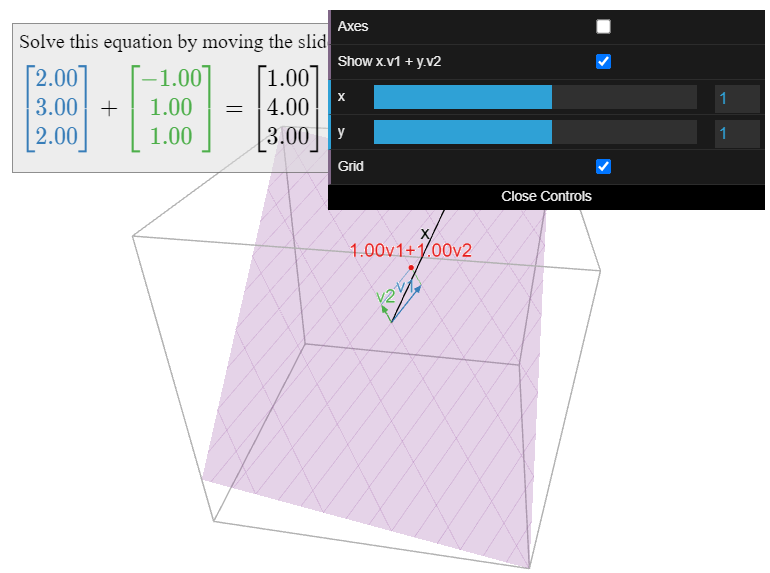
Figure $\PageIndex{6}$: A picture of the plane $V$ and the basis $\mathcal{B}=\{v_1,\:v_2\}$. The violet grid is a picture of the coordinate system defined by the basis $\mathcal{B}$; one set of lines measures the $v_1$-coordinate, and the other set measures the $v_2$-coordinate. Use the sliders to find the $\mathcal{B}$-coordinates of $x$.

Recipes: $\mathcal{B}$-Coordinates

If $\mathcal{B}=\{v_1,\: v_2,\cdots ,v_m\}$ is a basis for a subspace $V$ and $x$ is in $V$, then

$$[x]_{\mathcal{B}}=\left(\begin{array}{c}c_1 \\ c_2 \\ \vdots \\ c_m\end{array}\right)\quad\text{means}\quad x=c_1v_1+c_2v_2+\cdots c_mv_m.\nonumber$$

Finding the $\mathcal{B}$-coordinates of $x$ means solving the vector equation

$$x=c_1v_1+c_2v_2+\cdots +c_mv_m\nonumber$$

in the unknowns $c_1,\: c_2,\cdots ,c_m$. This generally means row reducing the augmented matrix

$$\left(\begin{array}{cccc|c} |&|&\quad&|&| \\ v_1&v_2&\quad &v_m&x \\ |&|&\quad &|&|\end{array}\right).\nonumber$$

Remark

Let $\mathcal{B}=\{v_1,\: v_2,\cdots ,v_m\}$ be a basis of a subspace $V$. Finding the $\mathcal{B}$-coordinates of a vector $x$ means solving the vector equation

$$x=c_1v_1+c_2v_2+\cdots +c_mv_m.\nonumber$$

If $x$ is not in $V$, then this equation has no solution, as $x$ is not in $V=\text{Span}\{v_1,\: v_2,\cdots ,v_m\}$. In other words, the above equation is inconsistent when $x$ is not in $V$.