
4.2: Finding zeros, maxima, and minima
- Page ID
- 48969

\( \newcommand{\vecs}[1]{\overset { \scriptstyle \rightharpoonup} {\mathbf{#1}} } \)
\( \newcommand{\vecd}[1]{\overset{-\!-\!\rightharpoonup}{\vphantom{a}\smash {#1}}} \)
\( \newcommand{\id}{\mathrm{id}}\) \( \newcommand{\Span}{\mathrm{span}}\)
( \newcommand{\kernel}{\mathrm{null}\,}\) \( \newcommand{\range}{\mathrm{range}\,}\)
\( \newcommand{\RealPart}{\mathrm{Re}}\) \( \newcommand{\ImaginaryPart}{\mathrm{Im}}\)
\( \newcommand{\Argument}{\mathrm{Arg}}\) \( \newcommand{\norm}[1]{\| #1 \|}\)
\( \newcommand{\inner}[2]{\langle #1, #2 \rangle}\)
\( \newcommand{\Span}{\mathrm{span}}\)
\( \newcommand{\id}{\mathrm{id}}\)
\( \newcommand{\Span}{\mathrm{span}}\)
\( \newcommand{\kernel}{\mathrm{null}\,}\)
\( \newcommand{\range}{\mathrm{range}\,}\)
\( \newcommand{\RealPart}{\mathrm{Re}}\)
\( \newcommand{\ImaginaryPart}{\mathrm{Im}}\)
\( \newcommand{\Argument}{\mathrm{Arg}}\)
\( \newcommand{\norm}[1]{\| #1 \|}\)
\( \newcommand{\inner}[2]{\langle #1, #2 \rangle}\)
\( \newcommand{\Span}{\mathrm{span}}\) \( \newcommand{\AA}{\unicode[.8,0]{x212B}}\)
\( \newcommand{\vectorA}[1]{\vec{#1}} % arrow\)
\( \newcommand{\vectorAt}[1]{\vec{\text{#1}}} % arrow\)
\( \newcommand{\vectorB}[1]{\overset { \scriptstyle \rightharpoonup} {\mathbf{#1}} } \)
\( \newcommand{\vectorC}[1]{\textbf{#1}} \)
\( \newcommand{\vectorD}[1]{\overrightarrow{#1}} \)
\( \newcommand{\vectorDt}[1]{\overrightarrow{\text{#1}}} \)
\( \newcommand{\vectE}[1]{\overset{-\!-\!\rightharpoonup}{\vphantom{a}\smash{\mathbf {#1}}}} \)
\( \newcommand{\vecs}[1]{\overset { \scriptstyle \rightharpoonup} {\mathbf{#1}} } \)
\( \newcommand{\vecd}[1]{\overset{-\!-\!\rightharpoonup}{\vphantom{a}\smash {#1}}} \)
\(\newcommand{\avec}{\mathbf a}\) \(\newcommand{\bvec}{\mathbf b}\) \(\newcommand{\cvec}{\mathbf c}\) \(\newcommand{\dvec}{\mathbf d}\) \(\newcommand{\dtil}{\widetilde{\mathbf d}}\) \(\newcommand{\evec}{\mathbf e}\) \(\newcommand{\fvec}{\mathbf f}\) \(\newcommand{\nvec}{\mathbf n}\) \(\newcommand{\pvec}{\mathbf p}\) \(\newcommand{\qvec}{\mathbf q}\) \(\newcommand{\svec}{\mathbf s}\) \(\newcommand{\tvec}{\mathbf t}\) \(\newcommand{\uvec}{\mathbf u}\) \(\newcommand{\vvec}{\mathbf v}\) \(\newcommand{\wvec}{\mathbf w}\) \(\newcommand{\xvec}{\mathbf x}\) \(\newcommand{\yvec}{\mathbf y}\) \(\newcommand{\zvec}{\mathbf z}\) \(\newcommand{\rvec}{\mathbf r}\) \(\newcommand{\mvec}{\mathbf m}\) \(\newcommand{\zerovec}{\mathbf 0}\) \(\newcommand{\onevec}{\mathbf 1}\) \(\newcommand{\real}{\mathbb R}\) \(\newcommand{\twovec}[2]{\left[\begin{array}{r}#1 \\ #2 \end{array}\right]}\) \(\newcommand{\ctwovec}[2]{\left[\begin{array}{c}#1 \\ #2 \end{array}\right]}\) \(\newcommand{\threevec}[3]{\left[\begin{array}{r}#1 \\ #2 \\ #3 \end{array}\right]}\) \(\newcommand{\cthreevec}[3]{\left[\begin{array}{c}#1 \\ #2 \\ #3 \end{array}\right]}\) \(\newcommand{\fourvec}[4]{\left[\begin{array}{r}#1 \\ #2 \\ #3 \\ #4 \end{array}\right]}\) \(\newcommand{\cfourvec}[4]{\left[\begin{array}{c}#1 \\ #2 \\ #3 \\ #4 \end{array}\right]}\) \(\newcommand{\fivevec}[5]{\left[\begin{array}{r}#1 \\ #2 \\ #3 \\ #4 \\ #5 \\ \end{array}\right]}\) \(\newcommand{\cfivevec}[5]{\left[\begin{array}{c}#1 \\ #2 \\ #3 \\ #4 \\ #5 \\ \end{array}\right]}\) \(\newcommand{\mattwo}[4]{\left[\begin{array}{rr}#1 \amp #2 \\ #3 \amp #4 \\ \end{array}\right]}\) \(\newcommand{\laspan}[1]{\text{Span}\{#1\}}\) \(\newcommand{\bcal}{\cal B}\) \(\newcommand{\ccal}{\cal C}\) \(\newcommand{\scal}{\cal S}\) \(\newcommand{\wcal}{\cal W}\) \(\newcommand{\ecal}{\cal E}\) \(\newcommand{\coords}[2]{\left\{#1\right\}_{#2}}\) \(\newcommand{\gray}[1]{\color{gray}{#1}}\) \(\newcommand{\lgray}[1]{\color{lightgray}{#1}}\) \(\newcommand{\rank}{\operatorname{rank}}\) \(\newcommand{\row}{\text{Row}}\) \(\newcommand{\col}{\text{Col}}\) \(\renewcommand{\row}{\text{Row}}\) \(\newcommand{\nul}{\text{Nul}}\) \(\newcommand{\var}{\text{Var}}\) \(\newcommand{\corr}{\text{corr}}\) \(\newcommand{\len}[1]{\left|#1\right|}\) \(\newcommand{\bbar}{\overline{\bvec}}\) \(\newcommand{\bhat}{\widehat{\bvec}}\) \(\newcommand{\bperp}{\bvec^\perp}\) \(\newcommand{\xhat}{\widehat{\xvec}}\) \(\newcommand{\vhat}{\widehat{\vvec}}\) \(\newcommand{\uhat}{\widehat{\uvec}}\) \(\newcommand{\what}{\widehat{\wvec}}\) \(\newcommand{\Sighat}{\widehat{\Sigma}}\) \(\newcommand{\lt}{<}\) \(\newcommand{\gt}{>}\) \(\newcommand{\amp}{&}\) \(\definecolor{fillinmathshade}{gray}{0.9}\)In this section, we will show how to locate local maxima and minima of a function (peaks and valleys of its graph), and the intersection points of two graphs. Further we will be able to use the calculator to find the \(x\)-intercepts of a graph. The \(x\)-intercepts are commonly called zeros or roots of the function \(f\). In other words, a zero of a function \(f\) is a number \(x\) for which \(f(x)=0\).
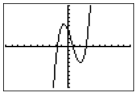
Graph the equation \(y=x^3-2x^2-4x+4\).
- Find points on the graph via the trace function, and by using the table menu.
- Approximate the zeros of the function via the calculate menu, that is, approximate the \(x-\)coordinate(s) of the point(s) where the graph crosses the \(x-\)axis.
- Approximate the (local) maximum and minimum via the calculate menu. (A (local) maximum or minimum is also called an (local) extremum.)
Solution
- Graphing the function in the standard window gives the following graph:
Pressing \(\boxed {\text{trace} }\), we can move a cursor to the right and left via \(\boxed {\triangleright }\) and \(\boxed {\triangleleft }\). We can see several function values as displayed below:
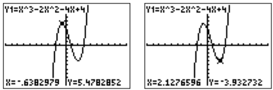
For the graph on the left we have displayed the point \((x,y)\approx\)\((-.638,5.478)\), and for the graph on the right, we have displayed the point \((x,y)\approx (2.128,-3.933)\).
Another way to find function values is to look at the table menu by pressing \(\boxed {2\text{nd} }\)\(\boxed {\text{graph} }\):
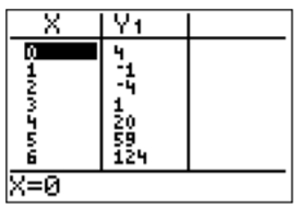
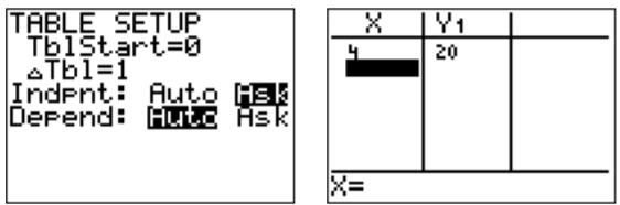
We see the \(y\)-values for specific \(x\)-values are displayed. More values can be displayed by pressing \(\boxed {\bigtriangleup }\) and \(\boxed {\bigtriangledown }\). Furthermore, the settings for the table can be changed in the table-set menu by pressing . In particular, by changing the the “Indpnt” setting in the table-set menu from “Auto” to “Ask”, we can have specific values calculated in the table menu. For example, below, we have calculated the value of \(y\) for the independent variable \(x\) set to \(x=4\).
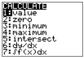
- Note, that the function \(f\) has three \(x\)-intercepts (the places on a graph intersects with the \(x\)-axis). They are called the zeros of the function and can be approximated with the TI-84. We have to find each zero, one at a time. To this end, we need to switch the calculate menu \(\boxed {2\text{nd} }\)\(\boxed {\text{trace} }\):

Press \(\boxed {2}\) to find a zero. We need to specify a left bound (using the keys \(\boxed {\triangleleft }\), \(\boxed {\triangleright }\) and \(\boxed {\text{enter} }\)), that is a point on the graph that is a bit left of the zero that we seek. Next, we also need to specify a right bound for our zero, and also a “guess” that is close to the zero:
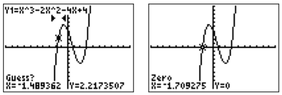
The zero displayed is approximately at \(x\approx -1.709\) (rounded to the nearest thousandth).
Similarly, we can also approximate the other zeros using the calculate menu \(\boxed {2\text{nd} }\)\(\boxed {\text{trace} }\). After choosing lower bounds, upper bounds, and guesses, we obtain:
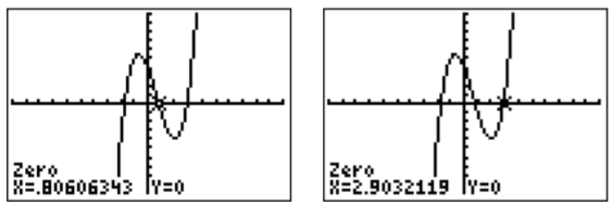
The zeros are approximately at \(x\approx 0.806\) and \(x\approx 2.903\).
- The TI-84 can also approximate the maximum and minimum of the function (the places on a graph where there is a ’peak’ or a ’valley’). This is again done in the calculate menu \(\boxed {2\text{nd} }\)\(\boxed {\text{trace} }\):
Now, press \(\boxed {3}\) for the minimum. After specifying a left bound, a right bound, and a guess, we obtain the following answer for our minimum:
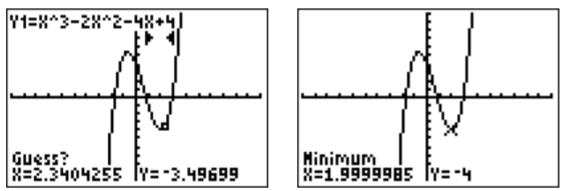
The minimum displayed is at \((1.9999985,-4)\). The actual answer on your calculator may be different, depending on the bounds and the guess chosen. However, it is important to note that the exact minimum is at \((x,y)=(2,-4)\), whereas the calculator only provides an approximation of the minimum!
Similarly, we can also approximate the maximum in the calculate menu \(\boxed {2\text{nd} }\)\(\boxed {\text{trace} }\)\(\boxed {4}\). After choosing lower and upper bound, we obtain:
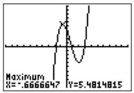
Therefore, the maximum is approximately at \((x,y)\approx (-0.667, 5.481)\), after rounding to the nearest thousandth.
This concludes the example.
We can always return to the home screen by pressing quit, that is \(\boxed {2\text{nd} }\)\(\boxed {\text{mode} }\).
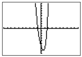
Graph the equation \(y=x^4-x^3-4x^2+4x\).
- Approximate the zeros of the function via the calculate menu.
- Approximate the (local) maxima and the minima via the calculate menu.
- Calculate the zeros of the function via the solve function.
Solution
- First, press \(\boxed {y= }\)and enter the function \(y=x^4-x^3-4x^2+4x\). We find the zeros using item \(2\) from the calculate menu. Here are two of the four zeros:
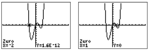
Note, in particular, the left zero has a \(y\) value of “\(1.6\)E\(-12\),” that is \(y=1.6\cdot 10^{-12}=0.0000000000016\). The value \(x=-2\) is an actual zero as can be seen by direct computation, whereas the calculator only obtains an approximation!
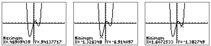
- From the calculate menu, \(\boxed {2\text{nd} }\)\(\boxed {\text{trace} }\), items \(3\) and \(4\) can be used to approximate the maximum and the two minima, (choosing a lower bound, upper bound, and a guess each time):
- There is also a non-graphical procedure to calculate the zeros of the function \(y=x^4-x^3-4x^2+4x\). Algebraically, we want to find a number \(x\) so that \(y=0\). In other words:
\[0=x^4-x^3-4x^2+4x \nonumber \]
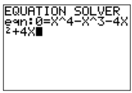
Press the \(\boxed {\text{math} }\) button, scroll down to “Solver...” and press the \(\boxed {\text{enter} }\) key. You will end up in one of the following two screens:
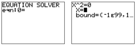
If you obtained the screen on the right, press \(\boxed {\bigtriangleup }\) to get to the screen on the left. Enter the equation and press \(\boxed {\text{enter} }\).
We now need to specify a number \(X\) which is our “guess” for the zero. In other words, the calculator will try to identify a zero that is close to a specified number \(X\). For example, we may enter \(x=3\). Then, the solve command is executed by pressing \(\boxed {\text{alpha} }\)\(\boxed {\text{enter} }\); (the \(\boxed {\text{alpha} }\)-key gives access to the commands written in green). We obtain the following zero:
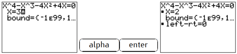
Choosing other values for \(x\) (for example \(x=1.2\), \(x=0.2\) and \(x=-3\)) produces the other three zeros after pressing \(\boxed {\text{alpha} }\)\(\boxed {\text{enter} }\).
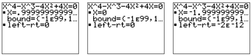
Note, that the exact zeros are \(x=2\), \(x=1\), \(x=0\), and \(x=-2\), whereas again the calculator only supplied an approximation!
The equation solver used in the last example (part (c)) is a slightly faster method for finding zeros than using the graph and the calculate menu. However, the disadvantage is that we first need to have some knowledge about the zeros (such as how many zeros there are!) before we can effectively use this tool. Generally, the graph and the calculate menu will give us a much better idea of where the zeros are located. For this reason, we recommend to use the calculate menu as the main method of finding zeros.
Solve the equation. Approximate your answer to the nearest hundredth.
- \(x^{4}+3 x^{2}-5 x-7=0\)
- \(x^{3}-4=7 x-3^{x}\)
Solution
- We need to find all numbers \(x\) so that \(x^4+3x^2-5x-7=0\). Note, that these are precisely the zeros of the function \(f(x)=x^4+3x^2-5x-7\), since the zeros are the values \(x\) for which \(f(x)=0\). Graphing the function \(f(x)=x^4+3x^2-5x-7\) shows that there are two zeros.
Using the calculate menu, we can identify both zeros.
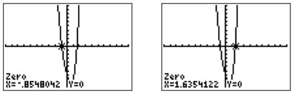
The answer is therefore, \(x\approx -0.85\) and \(x\approx 1.64\) (rounded to the nearest hundredth).
- We use the same method as in part (a). To this end we rewrite the equation so that one side becomes zero: \[x^3-4-7x+3^x=0 \nonumber \]We can now graph the function \(f(x)=x^3-4-7x+3^x\) and find its zeros.
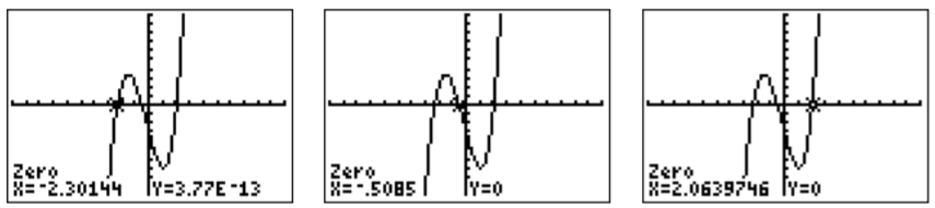
We see that there are three solutions, \(x\approx -2.30\), \(x\approx -0.51\), and \(x\approx 2.06\).
By a method similar to the above, we can also find the intersection points of two given graphs.
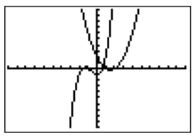
Graph the equations: \(y=x^2-3x+2\) and \(y=x^3+2x^2-1\).
- Approximate the intersection point of the two graphs via the calculate menu.
- Calculate the intersection point of the two graphs via the solve function.
Solution
First, enter the two equations for Y1 and Y2 after pressing \(\boxed {y= }\) the key. Both graphs are displayed in the graphing window.
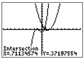
- The procedure for finding the intersection of the graphs for Y1 and Y2 is similar to finding minima, maxima, or zeros. In the calculate menu, \(\boxed {2\text{nd} }\)\(\boxed {\text{trace} }\), choose intersect (item 5). Choose the first curve Y1 (with \(\boxed {\bigtriangleup }\), \(\boxed {\bigtriangledown }\) and \(\boxed {\text{enter} }\))), and the second curve Y2. Finally choose a guess of the intersection point (with \(\boxed {\triangleleft }\), \(\boxed {\triangleright }\) and \(\boxed {\text{enter} }\))). The intersection is approximated as \((x,y)\approx (.71134574,.37197554)\):
- The intersection is the point where the two \(y\)-values \(y=x^2-3x+2\) and \(y=x^3+2x^2-1\) coincide. Therefore, we want to find an \(x\) with
\[x^2-3x+2=x^3+2x^2-1 \nonumber \]
The TI-84 equation solver requires an equation with zero on the left. Therefore, we subtract the left-hand side, and obtain:
\[\begin{aligned} \text{(subtract $(x^2-3x+2)$)} & \implies & 0 = (x^3+2x^2-1)-(x^2-3x+2) \\ & \implies & 0 = \,\, x^3+2x^2-1\,\,\, -\,\, x^2+3x-2 \\ & \implies & 0 = x^3+x^2+3x-3\end{aligned} \nonumber \]
Entering \(0=x^3+x^2+3x-3\) into the equation solver, , and choosing an approximation \(x=1\) for X, the calculator solves this equation (using \(\boxed {\text{alpha} }\)\(\boxed {\text{enter} }\)) as follows:
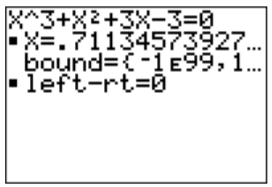
The approximation provided by the calculator is \(x\approx .71134573927\dots\).