16.2: Compound Interest

There is another interesting and important application of the exponential function given by calculating the interest on an investment. We start with the following motivating example.

Example \(\PageIndex{1}\)

• We invest an initial amount of \(P=\$500\) for \(1\) year at a rate of \(r=6\%\). The initial amount \(P\) is also called the principal.

  After \(1\) year, we receive the principal \(P\) together with the interest \(r\cdot P\) generated from the principal. The final amount \(A\) after \(1\) year is therefore

  \[A=\$ 500+ 6\%\cdot \$ 500=\$500 \cdot(1+0.06)= \$ 530 \nonumber \]

• We change the setup of the previous example by taking a quarterly compounding. This means, that instead of receiving interest on the principal once at the end of the year, we receive the interest \(4\) times within the year (after each quarter). However, we now receive only \(\dfrac{1}{4}\) of the interest rate of \(6\%\). We break down the amount received after each quarter.

  \[\begin{aligned}
  \text{after first quarter:} \quad 500\cdot \Big(1+\dfrac{0.06}{4}\Big)&={\color{Red} 500 \cdot 1.015} \\ \text{after second quarter:} \quad ({\color{Red} 500 \cdot 1.015})\cdot \Big(1+\dfrac{0.06}{4}\Big)&={\color{Blue} 500 \cdot 1.015^2} \\
  \text{after third quarter:} \quad ({\color{Blue}500 \cdot 1.015^2})\cdot \Big(1+\dfrac{0.06}{4}\Big)&={\color{Green}500 \cdot 1.015^3} \\
  \text{after fourth quarter:} \quad A&= ({\color{Green}500 \cdot 1.015^3})\cdot \Big(1+\dfrac{0.06}{4}\Big)=500 \cdot 1.015^4 \\
  \implies A&\approx 530.68
  \end{aligned} \nonumber \]

  Note that in the second quarter, we receive interest on the amount we had after the first quarter, and so on. So, in fact, we keep receiving interest on the interest of the interest, etc. For this reason, the final amount received after \(1\) year \(A=\$ 530.68\) is slightly higher when compounded quarterly than when compounded annually (where \(A=\$ 530.00\)).

• We make an even further variation from the above. Instead of investing money for \(1\) year, we invest the principal for \(10\) years at a quarterly compounding. We then receive interest every quarter for a total of \(4\cdot 10=40\) quarters.

  \[\begin{aligned}
  \text{after first quarter:} \quad 500\cdot \Big(1+\dfrac{0.06}{4}\Big)&=500 \cdot 1.015 \\
  \text{after second quarter:} \quad (500 \cdot 1.015)\cdot \Big(1+\dfrac{0.06}{4}\Big)&=500 \cdot 1.015^2 \\ \quad &\vdots\\
  \text{after fortieth quarter:} \quad A&= (500 \cdot 1.015^{39})\cdot \Big(1+\dfrac{0.06}{4}\Big)=500 \cdot 1.015^{40} \\
  \implies A &\approx 907.01
  \end{aligned} \nonumber \]

We state our observations from the previous example in the following general observation.

Observation: \(n\)th-Compounding

A principal (=initial amount) \(P\) is invested for \(t\) years at a rate \(r\) and compounded \(n\) times per year. The final amount \(A\) is given by

\[\boxed {A=P \cdot\left(1+\frac{r}{n}\right)^{n \cdot t}} \text { where }\left\{\begin{array}{l}
P=\text { principal }(=\text { initial }) \text { amount } \\
A=\text { final amount } \\
r=\text { annual interest rate } \\
n=\text { number of compoundings per year } \\
t=\text { number of years }
\end{array}\right. \]

We can consider performing the compounding in smaller and smaller increments. Instead of quarterly compounding, we may take monthly compounding, or daily, hourly, secondly compounding or compounding in even smaller time intervals. Note, that in this case the number of compoundings \(n\) in the above formula tends to infinity. In the limit when the time intervals go to zero, we obtain what is called continuous compounding.

Observation: Continuous Compounding

A principal amount \(P\) is invested for \(t\) years at a rate \(r\) and with continuous compounding. The final amount \(A\) is given by

\[\boxed {A=P \cdot e^{r \cdot t}} \quad \text { where }\left\{\begin{array}{l}
P=\text { principal amount } \\
A=\text { final amount } \\
r=\text { annual interest rate } \\
t=\text { number of years }
\end{array}\right. \]

Note

The reason the exponential function appears in the above formula is that the exponential is the limit of the previous formula in observation \(n\)th-compounding, when \(n\) approaches infinity; compare this with equation 13.1.1.

\[e^r=\lim_{n\to \infty} \left(1+\dfrac r n\right)^n \nonumber \]

A more detailed discussion of limits (including its definition) will be provided in a calculus course.

Example \(\PageIndex{1}\)

Determine the final amount received on an investment under the given conditions.

1. \(\$700\), compounded monthly, at \(4\%\), for \(3\) years
2. \(\$2500\), compounded semi-annually, at \(5.5\%\), for \(6\) years
3. \(\$1200\), compounded continuously, at \(3\%\), for \(2\) years

Solution

We can immediately use the formula by substituting the given values.

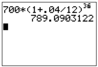
1. For part (a), we have \(P=700\), \(n=12\), \(r=4\%=0.04\), and \(t=3\). Therefore, we calculate

\[A=700\cdot\left(1+\dfrac{0.04}{12}\right)^{12\cdot 3}=700\cdot\left(1+\dfrac{0.04}{12}\right)^{36}\approx 789.09 \nonumber \]

2. We have \(P=2500\), \(n=2\), \(r=5.5\%=0.055\), and \(t=6\).

\[A=2500\cdot\left(1+\dfrac{0.055}{2}\right)^{2\cdot 6}\approx 3461.96 \nonumber \]

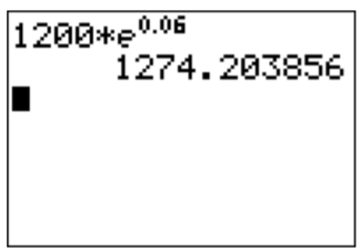
3. We have \(P=1200\), \(r=3\%=0.03\), \(t=2\), and we use the formula for continuous compounding.

\[A=1200\cdot e^{0.03\cdot 2}=1200 \cdot e^{0.06} \approx 1274.20 \nonumber \]

(Note that the Euler number is entered in the TI-84 via the keys and \(\boxed { \text {ln}}\).)

Instead of asking to find the final amount, we may also ask about any of the other variables in the above formulas for investments.

Example \(\PageIndex{1}\)

1. Find the amount \(P\) that needs to be invested at \(4.275 \%\) compounded annually for \(5\) years to give a final amount of \(\$ 3000\). (This amount \(P\) is also called the present value of the future amount of \(\$3000\) in \(5\) years.)
2. At what rate do we have to invest \(\$800\) for \(6\) years compounded quarterly to obtain a final amount of \(\$1200\)?
3. For how long do we have to invest \(\$1000\) at a rate of \(2.5 \%\) compounded continuously to obtain a final amount of \(\$1100\)?
4. For how long do we have to invest at a rate of \(3.2\%\) compounded monthly until the investment doubles its value?

Solution

1. We have the following data: \(r=4.275\%=0.04275\), \(n=1\), \(t=5\), and \(A=3000\). We want to find the present value \(P\). Substituting the given numbers into the appropriate formula, we can solve this for \(P\).

\[\begin{aligned}
3000&=P\cdot \left(1+\dfrac{0.04275}{1}\right)^{1\cdot 5}\\
\implies 3000&=P\cdot \left(1.04275\right)^{ 5} \\
\implies P&=\dfrac{3000}{1.04275^5}\approx 2433.44 \quad \text{(divide by $1.04275^5$)}
\end{aligned} \nonumber \]

Therefore, if we invest \(\$2433.44\) today under the given conditions, then this will be worth \(\$3000\) in \(5\) years.

2. Substituting the given numbers (\(P=800\), \(t=6\), \(n=4\), \(A=1200\)) into the formula gives:

\[\begin{aligned}
1200&=800\cdot \left(1+\dfrac{r}{4}\right)^{4\cdot 6}\\
\implies \dfrac{1200}{800}&= \left(1+\dfrac r 4\right)^{24} \quad \text{(divide by $800$)}\\
\implies \left(1+\dfrac r 4\right)^{24}&=\dfrac{3}{2}
\end{aligned} \nonumber \]

Next, we have to get the exponent \(24\) to the right side. This is done by taking a power of \(\dfrac{1}{24}\), or in other words, by taking the \(24\)th root, \(\sqrt[24]{\dfrac{3}{2}}=\Big(\dfrac{3}{2}\Big)^{\frac{1}{24}}\).

\[\begin{aligned}
\left(\left(1+\dfrac{r}{4}\right)^{24}\right)^{\frac{1}{24}}&=\left(\dfrac{3}{2}\right)^{\frac{1}{24}}\\
\implies \left(1+\dfrac{r}{4}\right)^{24\cdot \frac{1}{24}}&=\left(\dfrac{3}{2}\right)^{\frac{1}{24}} \\ \implies 1+\dfrac{r}{4}&=\left(\frac{3}{2}\right)^{\frac{1}{24}}\\
\implies \dfrac{r}{4}&=\left(\dfrac{3}{2}\right)^{\frac{1}{24}} -1 \\
\implies r&=4\cdot \left(\left(\dfrac{3}{2}\right)^{\frac{1}{24}} -1\right)
\end{aligned} \nonumber \]

We plug this into the calculator. Note that the \(n\)th root is given by pressing \(\boxed {\text{math}}\) and .

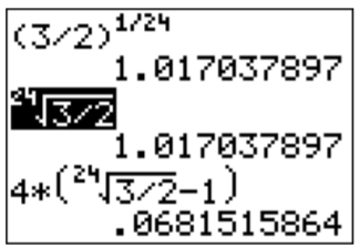
More precisely, the \(24\)th root of \(3/2\) (highlighted above) can be entered by pressing the following keys:

\(\boxed {2}\)\(\boxed {4}\) \(\boxed {\text{math}}\)\(\boxed {5}\) \(\boxed {3}\)\(\boxed {\div}\)\(\boxed {2}\) \(\boxed {\text{enter}}\)

Therefore our answer is \(r\approx 0.06815 =6.815\%\).

3. Again we substitute the given values, \(P=1000\), \(r=2.5\%=0.025\), \(A=1100\), but now we use the formula for continuous compounding.

\[1100=1000\cdot e^{0.025\cdot t} \implies \quad \dfrac{1100}{1000}= e^{0.025\cdot t}\implies \quad e^{0.025\cdot t}=1.1 \nonumber \]

To solve for the variable \(t\) in the exponent, we need to apply the logarithm. Here, it is most convenient to apply the natural logarithm, because \(\ln(x)\) is inverse to \(e^x\) (which appears in the equation) and this logarithm is directly implemented on the calculator via the \(\boxed {\text{ln}}\) key. By applying \(\ln\) to both sides, since \(\ln(x)\) is inverse to \(e^x\), we see that \(.025 t=\ln(1.1)\).

Alternatively,

\[\ln(e^{0.025\cdot t})=\ln(1.1)\quad \implies \quad 0.025\cdot t\cdot \ln(e)=\ln(1.1) \nonumber \]

Here we have used that \(\log_b(x^n)=n\cdot \log_b(x)\) for any number \(n\) as we have seen in proposition logarithmic properties. Observing that \(\ln(e)=1\), which is the special case of the second equation in [elementary-log] on page for the base \(b=e\), the above becomes

\[0.025\cdot t=\ln(1.1) \quad \implies \quad t=\dfrac{\ln(1.1)}{0.025}\approx 3.81 \nonumber \]

Therefore, we have to wait \(4\) years until the investment is worth (more than) \(\$1100\).

4. We are given that \(r=3.2\%=0.032\) and \(n=12\), but no initial amount \(P\) is provided. We are seeking to find the time \(t\) when the investment doubles. This means that the final amount \(A\) is twice the initial amount \(P\), or as a formula: \(A=2\cdot P\). Substituting this into the investment formula and solving gives the wanted answer.

\[\begin{aligned}
2P&=P\cdot \left(1+\dfrac{0.032}{12}\right)^{12\cdot t}\\
\implies 2&= \left(1+\dfrac{0.032}{12}\right)^{12\cdot t} \qquad \text{(divide by $P$)}\\
\implies \quad \ln(2)&= \ln\left(\left(1+\dfrac{0.032}{12}\right)^{12\cdot t}\right) \qquad \text{(apply $\ln$)}\\
\implies \ln(2)&= 12\cdot t \cdot \ln\left(1+\dfrac{0.032}{12}\right)\\
\implies t&=\dfrac{\ln(2)}{12\cdot \ln\left(1+\dfrac{0.032}{12}\right)} \qquad \text{divide by)}12\cdot \ln\left(1+\dfrac{0.032}{12}\right)\\
&\approx 21.69
\end{aligned} \nonumber \]

So, after approximately \(21.69\) years, the investment will have doubled in value.