17.2: sin, cos, and tan as functions
- Page ID
- 49060

\( \newcommand{\vecs}[1]{\overset { \scriptstyle \rightharpoonup} {\mathbf{#1}} } \)
\( \newcommand{\vecd}[1]{\overset{-\!-\!\rightharpoonup}{\vphantom{a}\smash {#1}}} \)
\( \newcommand{\id}{\mathrm{id}}\) \( \newcommand{\Span}{\mathrm{span}}\)
( \newcommand{\kernel}{\mathrm{null}\,}\) \( \newcommand{\range}{\mathrm{range}\,}\)
\( \newcommand{\RealPart}{\mathrm{Re}}\) \( \newcommand{\ImaginaryPart}{\mathrm{Im}}\)
\( \newcommand{\Argument}{\mathrm{Arg}}\) \( \newcommand{\norm}[1]{\| #1 \|}\)
\( \newcommand{\inner}[2]{\langle #1, #2 \rangle}\)
\( \newcommand{\Span}{\mathrm{span}}\)
\( \newcommand{\id}{\mathrm{id}}\)
\( \newcommand{\Span}{\mathrm{span}}\)
\( \newcommand{\kernel}{\mathrm{null}\,}\)
\( \newcommand{\range}{\mathrm{range}\,}\)
\( \newcommand{\RealPart}{\mathrm{Re}}\)
\( \newcommand{\ImaginaryPart}{\mathrm{Im}}\)
\( \newcommand{\Argument}{\mathrm{Arg}}\)
\( \newcommand{\norm}[1]{\| #1 \|}\)
\( \newcommand{\inner}[2]{\langle #1, #2 \rangle}\)
\( \newcommand{\Span}{\mathrm{span}}\) \( \newcommand{\AA}{\unicode[.8,0]{x212B}}\)
\( \newcommand{\vectorA}[1]{\vec{#1}} % arrow\)
\( \newcommand{\vectorAt}[1]{\vec{\text{#1}}} % arrow\)
\( \newcommand{\vectorB}[1]{\overset { \scriptstyle \rightharpoonup} {\mathbf{#1}} } \)
\( \newcommand{\vectorC}[1]{\textbf{#1}} \)
\( \newcommand{\vectorD}[1]{\overrightarrow{#1}} \)
\( \newcommand{\vectorDt}[1]{\overrightarrow{\text{#1}}} \)
\( \newcommand{\vectE}[1]{\overset{-\!-\!\rightharpoonup}{\vphantom{a}\smash{\mathbf {#1}}}} \)
\( \newcommand{\vecs}[1]{\overset { \scriptstyle \rightharpoonup} {\mathbf{#1}} } \)
\( \newcommand{\vecd}[1]{\overset{-\!-\!\rightharpoonup}{\vphantom{a}\smash {#1}}} \)
\(\newcommand{\avec}{\mathbf a}\) \(\newcommand{\bvec}{\mathbf b}\) \(\newcommand{\cvec}{\mathbf c}\) \(\newcommand{\dvec}{\mathbf d}\) \(\newcommand{\dtil}{\widetilde{\mathbf d}}\) \(\newcommand{\evec}{\mathbf e}\) \(\newcommand{\fvec}{\mathbf f}\) \(\newcommand{\nvec}{\mathbf n}\) \(\newcommand{\pvec}{\mathbf p}\) \(\newcommand{\qvec}{\mathbf q}\) \(\newcommand{\svec}{\mathbf s}\) \(\newcommand{\tvec}{\mathbf t}\) \(\newcommand{\uvec}{\mathbf u}\) \(\newcommand{\vvec}{\mathbf v}\) \(\newcommand{\wvec}{\mathbf w}\) \(\newcommand{\xvec}{\mathbf x}\) \(\newcommand{\yvec}{\mathbf y}\) \(\newcommand{\zvec}{\mathbf z}\) \(\newcommand{\rvec}{\mathbf r}\) \(\newcommand{\mvec}{\mathbf m}\) \(\newcommand{\zerovec}{\mathbf 0}\) \(\newcommand{\onevec}{\mathbf 1}\) \(\newcommand{\real}{\mathbb R}\) \(\newcommand{\twovec}[2]{\left[\begin{array}{r}#1 \\ #2 \end{array}\right]}\) \(\newcommand{\ctwovec}[2]{\left[\begin{array}{c}#1 \\ #2 \end{array}\right]}\) \(\newcommand{\threevec}[3]{\left[\begin{array}{r}#1 \\ #2 \\ #3 \end{array}\right]}\) \(\newcommand{\cthreevec}[3]{\left[\begin{array}{c}#1 \\ #2 \\ #3 \end{array}\right]}\) \(\newcommand{\fourvec}[4]{\left[\begin{array}{r}#1 \\ #2 \\ #3 \\ #4 \end{array}\right]}\) \(\newcommand{\cfourvec}[4]{\left[\begin{array}{c}#1 \\ #2 \\ #3 \\ #4 \end{array}\right]}\) \(\newcommand{\fivevec}[5]{\left[\begin{array}{r}#1 \\ #2 \\ #3 \\ #4 \\ #5 \\ \end{array}\right]}\) \(\newcommand{\cfivevec}[5]{\left[\begin{array}{c}#1 \\ #2 \\ #3 \\ #4 \\ #5 \\ \end{array}\right]}\) \(\newcommand{\mattwo}[4]{\left[\begin{array}{rr}#1 \amp #2 \\ #3 \amp #4 \\ \end{array}\right]}\) \(\newcommand{\laspan}[1]{\text{Span}\{#1\}}\) \(\newcommand{\bcal}{\cal B}\) \(\newcommand{\ccal}{\cal C}\) \(\newcommand{\scal}{\cal S}\) \(\newcommand{\wcal}{\cal W}\) \(\newcommand{\ecal}{\cal E}\) \(\newcommand{\coords}[2]{\left\{#1\right\}_{#2}}\) \(\newcommand{\gray}[1]{\color{gray}{#1}}\) \(\newcommand{\lgray}[1]{\color{lightgray}{#1}}\) \(\newcommand{\rank}{\operatorname{rank}}\) \(\newcommand{\row}{\text{Row}}\) \(\newcommand{\col}{\text{Col}}\) \(\renewcommand{\row}{\text{Row}}\) \(\newcommand{\nul}{\text{Nul}}\) \(\newcommand{\var}{\text{Var}}\) \(\newcommand{\corr}{\text{corr}}\) \(\newcommand{\len}[1]{\left|#1\right|}\) \(\newcommand{\bbar}{\overline{\bvec}}\) \(\newcommand{\bhat}{\widehat{\bvec}}\) \(\newcommand{\bperp}{\bvec^\perp}\) \(\newcommand{\xhat}{\widehat{\xvec}}\) \(\newcommand{\vhat}{\widehat{\vvec}}\) \(\newcommand{\uhat}{\widehat{\uvec}}\) \(\newcommand{\what}{\widehat{\wvec}}\) \(\newcommand{\Sighat}{\widehat{\Sigma}}\) \(\newcommand{\lt}{<}\) \(\newcommand{\gt}{>}\) \(\newcommand{\amp}{&}\) \(\definecolor{fillinmathshade}{gray}{0.9}\)We now turn to function theoretic aspects of the trigonometric functions defined in the last section. In particular, we will be interested in understanding the graphs of the functions \(y=\sin(x)\), \(y=\cos(x)\), and \(y=\tan(x)\). With an eye toward calculus, we will take the angles \(x\) in radian measure.
We graph the functions \(y=\sin(x)\), \(y=\cos(x)\), and \(y=\tan(x)\).
Solution
One way to proceed is to calculate and collect various function values in a table and then graph them. However, this is quite elaborate, as the following table shows.
\[\begin{array}{c||c|c|c|c|c|c|c|c|c|c}
x & 0 & \dfrac{\pi}{6} & \dfrac{\pi}{4} & \dfrac{\pi}{3} & \dfrac{\pi}{2} & \dfrac{2 \pi}{3} & \dfrac{3 \pi}{4} & \dfrac{5 \pi}{6} & \pi & \ldots \\
\hline \hline \sin (x) & 0 & \dfrac{1}{2} & \dfrac{\sqrt{2}}{2} & \dfrac{\sqrt{3}}{2} & 1 & \dfrac{\sqrt{3}}{2} & \dfrac{\sqrt{2}}{2} & \dfrac{1}{2} & 0 & \ldots \\
\hline \cos (x) & 1 & \dfrac{\sqrt{3}}{2} & \dfrac{\sqrt{2}}{2} & \dfrac{1}{2} & 0 & \dfrac{-1}{2} & \dfrac{-\sqrt{2}}{2} & \dfrac{-\sqrt{3}}{2} & -1 & \ldots \\
\hline \tan (x) & 0 & \dfrac{\sqrt{3}}{3} & 1 & \sqrt{3} & \text { undef. } & -\sqrt{3} & -1 & \dfrac{-\sqrt{3}}{3} & 0 & \ldots
\end{array} \nonumber \]
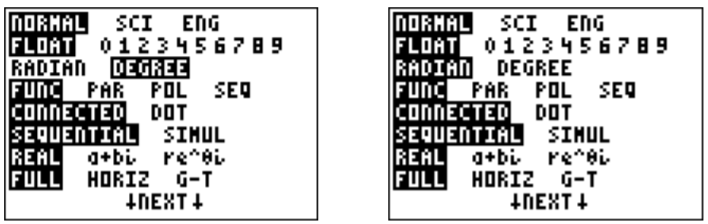
An easier approach is to use the TI-84 to graph each function. Before entering the function, we need to make sure that the calculator is in radian mode. For this, press the \(\boxed{\text{mode}}\) key, and in case the third item is set on degree, switch to radian, and press \(\boxed{\text{enter}}\).
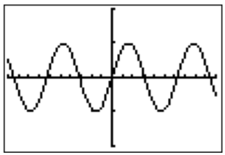
We may now enter the function \(y=\sin(x)\) and study its graph.

From this, we can make some immediate observations (which can also be seen using definition sin-cos-tan). First, the graph is bounded between \(-1\) and \(+1\), because by definition sin-cos-tan, we have \(\sin(x)=\dfrac b r\) with \(-r\leq b \leq r\), so that
\[-1\leq \sin(x)\leq 1, \quad \text{ for all }x \nonumber \]
We therefore change the window of the graph to display \(y\)’s between \(-2\) and \(2\), to get a closer view.
\(y=\sin (x)\)
Second, we see that \(y=\sin(x)\) is a periodic function with period \(2\pi\), since the function doesn’t change its value when adding \(360^\circ=2\pi\) to its argument (and this is the smallest non-zero number with that property):
\[\sin(x+2\pi)=\sin(x) \nonumber \]
The graph of \(y=\sin(x)\) has the following specific values:
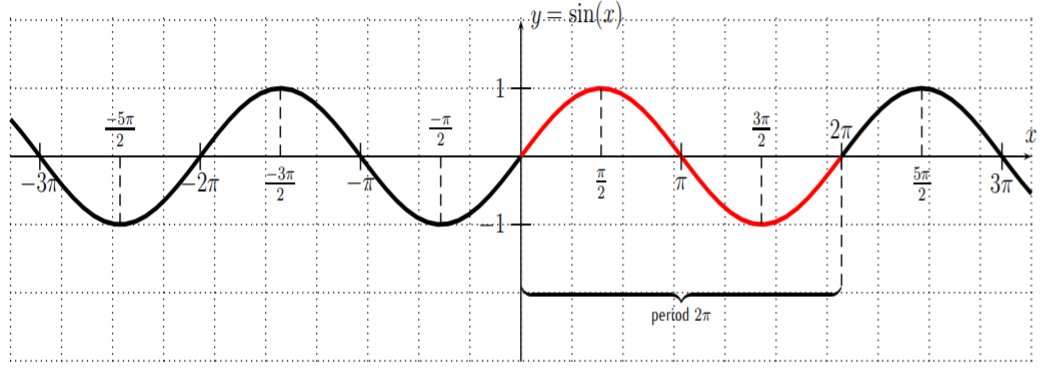
The graph of \(y=\sin(x)\) has a period of \(2\pi\), and an amplitude of \(1\).
Similarly, we can graph the function \(y=\cos(x)\). Since \(-1\leq \cos(x)\leq 1\) for all \(x\), we graph it also with the zoomed window setting.

\(y=\cos (x)\)
We see that \(y=\cos(x)\) is also periodic with period \(2\pi\), that is \[\cos(x+2\pi)=\cos(x) \nonumber \] and \(y=\cos(x)\) also has an amplitude of \(1\), since \(-1\leq\cos(x)\leq 1\).
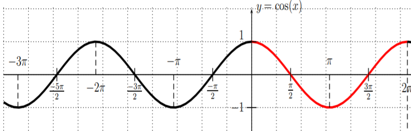
Indeed, the graph of \(y=\cos(x)\) is that of \(y=\sin(x)\) shifted to the left by \(\dfrac{\pi}{2}\). The reason for this is that
\[\label{EQ:cos=sin+pi2} \boxed{\cos(x)=\sin\left(x+\dfrac{\pi}{2}\right)} \]
Many other properties of \(\sin\) and \(\cos\) can be observed from the graph (or from the unit circle definition). For example, recalling Observation even-odd from page , we see that the sine function is an odd function, since the graph of \(y=\sin(x)\) is symmetric with respect to the origin. Similarly, the cosine function is an even function, since the graph of \(y=\cos(x)\) is symmetric with respect to the \(y\)-axis. Algebraically, Definition even-odd from page therefore shows that these functions satisfy the following relations:
\[\label{EQ:sin-odd-cos-even} \boxed{\sin(-x)=-\sin(x)} \quad\text{and}\quad \boxed{\cos(-x)=\cos(x)} \]
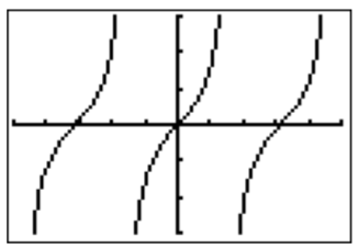
Finally, we come to the graph of \(y=\tan(x)\). Graphing this function in the standard window, we obtain:

\(y=\tan (x)\)
Zooming into this graph, we see that \(y=\tan(x)\) has vertical asymptotes \(x=\dfrac{\pi}{2}\approx 1.6\) and \(x=\dfrac{-\pi}{2}\approx-1.6\).
\(y=\tan (x)\)
This is also supported by the fact that \(\tan \left(\dfrac{\pi}{2} \right)\) and \(\tan \left(-\dfrac{\pi}{2} \right)\) are undefined. The graph of \(y=\tan(x)\) with some more specific function values is shown below.
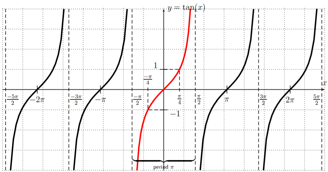
We see that the tangent is periodic with a period of \(\pi\):
\[\label{EQU:tan-period} \tan(x+\pi)=\tan(x) \nonumber \]
There are vertical asymptotes: \(x=\dfrac{\pi}{2}, \dfrac{-\pi}{2}, \dfrac{3\pi}{2}, \dfrac{-3\pi}{2}, \dfrac{5\pi}{2}, \dfrac{-5\pi}{2}, \dots\), or, in short
\[\text{asymptotes of }y=\tan(x): \quad x=n\cdot \dfrac{\pi}{2}, \text{ where }n=\pm1, \pm3, \pm5, \dots \nonumber\]
Furthermore, the tangent is an odd function, since it is symmetric with respect to the origin (see Observation even-odd):
Recall from section 5.2 how changing the formula of a function affects the graph of the function, such as:
- the graph of \(c\cdot f(x)\) (for \(c>0\)) is the graph of \(f(x)\) stretched away from the \(x\)-axis by a factor \(c\) (or compressed when \(0<c<1\))
- the graph of \(f(c\cdot x)\) (for \(c>0\)) is the graph of \(f(x)\) compressed towards the \(y\)-axis by a factor \(c\) (or stretched away the \(y\)-axis when \(0<c<1\))
- graph of \(f(x)+c\) is the graph of \(f(x)\) shifted up by \(c\) (or down when \(c<0\))
- graph of \(f(x+c)\) is the graph of \(f(x)\) shifted to the left by \(c\) (or to the right when \(c<0\))
With this we can graph some variations of the basic trigonometric functions.
Graph the functions:
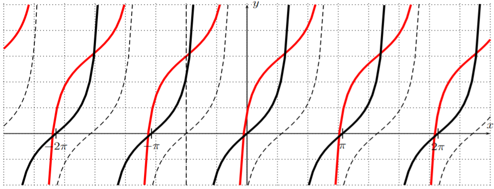
\[\begin{aligned} && f(x)=\sin(x)+3, \,\, g(x)=4\cdot \sin(x), \,\, h(x)=\sin(x+2), \,\, i(x)=\sin(3x), \\ && j(x)=2\cdot \cos(x)+3, \,\,\, k(x)=\cos(2x-\pi), \,\,\, l(x)=\tan(x+2)+3 \end{aligned} \nonumber \]
Solution
The functions \(f\), \(g\), \(h\), and \(i\) have graphs that are variations of the basic \(y=\sin(x)\) graph. The graph of \(f(x)=\sin(x)+3,\) shifts the graph of \(y=\sin(x)\) up by \(3\), whereas the graph of \(g(x)=4\cdot \sin(x)\) stretches \(y=\sin(x)\) away from the \(x\)-axis.
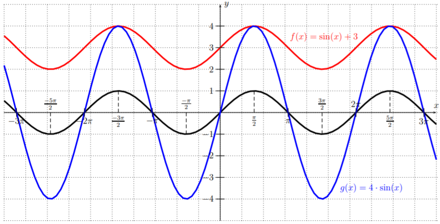
The graph of \(h(x)=\sin(x+2)\) shifts the graph of \(y=\sin(x)\) to the left by \(2\), and \(i(x)=\sin(3x)\) compresses \(y=\sin(x)\) towards the \(y\)-axis.

Next, \(j(x)=2\cdot \cos(x)+3\) has a graph of \(y=\cos(x)\) stretched by a factor \(2\) away from the \(x\)-axis, and shifted up by \(3\).

For the graph of \(k(x)=\cos(2x-\pi)=\cos\left(2\cdot \left(x-\dfrac{\pi}{2}\right)\right)\), we need to compress the graph of \(y=\cos(x)\) by a factor \(2\) (we obtain the graph of the function \(y=\cos(2x)\)) and then shift this by \(\dfrac{\pi}{2}\) to the right.
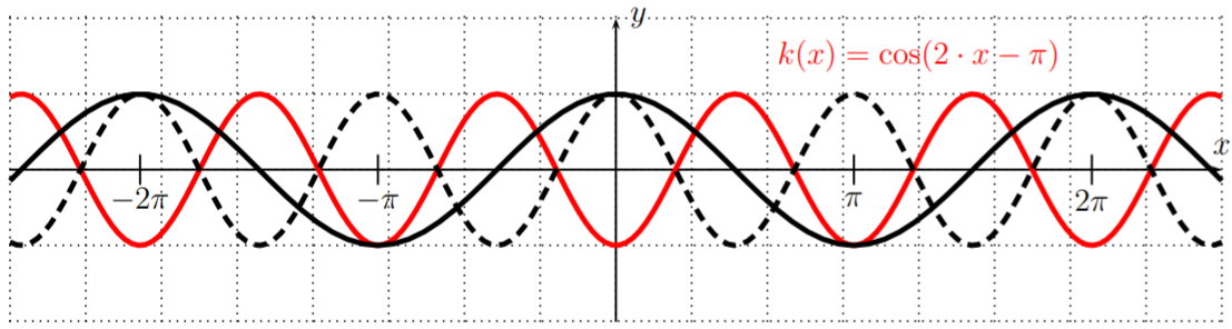
We will explore this case below in more generality. In fact, whenever \(y=\cos(b\cdot x +c)=\cos\Big(b\cdot \Big(x-\dfrac{-c}{b}\Big)\Big)\), the graph of \(y=\cos(x)\) is shifted to the right by \(\dfrac{-c}{b}\), and compressed by a factor \(b\), so that it has a period of \(\dfrac{2\pi}{b}\).
Finally, \(l(x)=\tan(x+2)+3\) shifts the graph of \(y=\tan(x)\) up by \(3\) and to the left by \(2\).
We collect some of the observations that were made in the above examples in the following definition.
Let \(f\) be one of the functions:
\[f(x)=a\cdot \sin(b\cdot x +c) \quad \text{or} \quad f(x)=a\cdot \cos(b\cdot x +c) \nonumber \]
The number \(|a|\) is called the amplitude, the number \(\left|\dfrac{2\pi}{b}\right|\) is the period, and the number \(\dfrac{-c}{b}\) is called the phase shift.
In physical applications, the period is sometimes denoted by \(T=\left|\dfrac{2\pi}{b}\right|\) and the frequency is the reciprocal \[f=\dfrac 1 T \nonumber \]
Using the amplitude, period and phase-shift, we can draw the graph of, for example, a function \(f(x)=a\cdot \sin(b\cdot x +c)\) over one period by shifting the graph of \(\sin(x)\) by the phase-shift \(\dfrac{-c}{b}\) to the right, then marking one full period of length \(\left|\dfrac{2\pi}{b}\right|\), and then drawing the basic \(\sin(x)\) graph with an amplitude of \(a\) (or the reflected graph of \(-\sin(x)\) when \(a\) is negative).
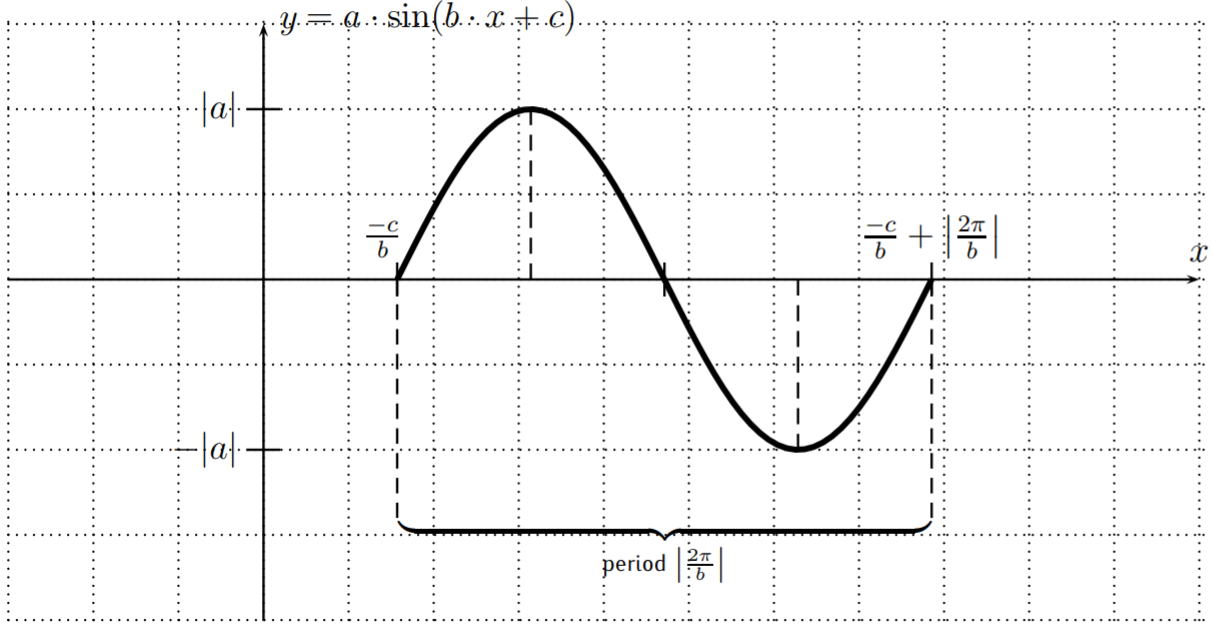
The zero(s), maxima, and minima of the graph within the drawn period can be found by calculating the midpoint between \(\left(\dfrac{-c}{b},0\right)\) and \(\left(\dfrac{-c}{b}+\dfrac{2\pi}{b},0\right)\) and midpoints between these and the resulting midpoint.
A similar graph can be obtained for \(f(x)=a\cdot \cos(b\cdot x +c)\) by replacing the \(\sin(x)\) graph with the \(\cos(x)\) graph over one period.
Find the amplitude, period, and phase-shift, and sketch the graph over one full period.
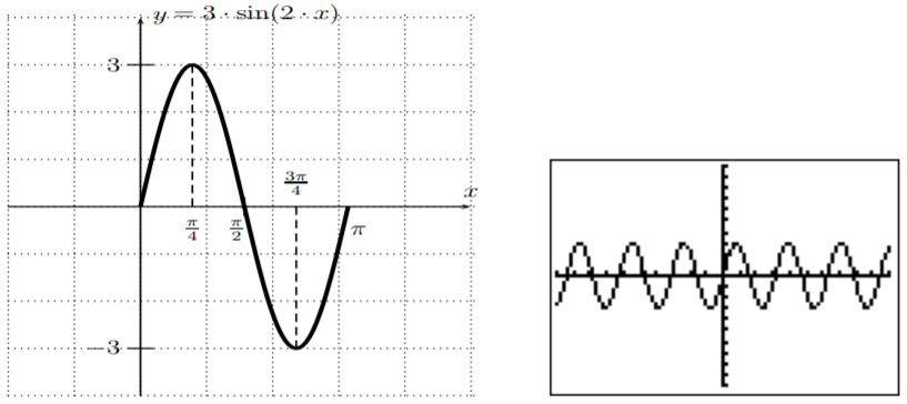
- \(f(x)=3 \sin(2 x)\)
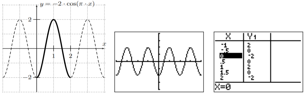
- \(f(x)=-2\cos(\pi\cdot x)\)
- \(f(x)=\cos(x-2)\)
- \(f(x)=\cos(2 x+\pi)\)
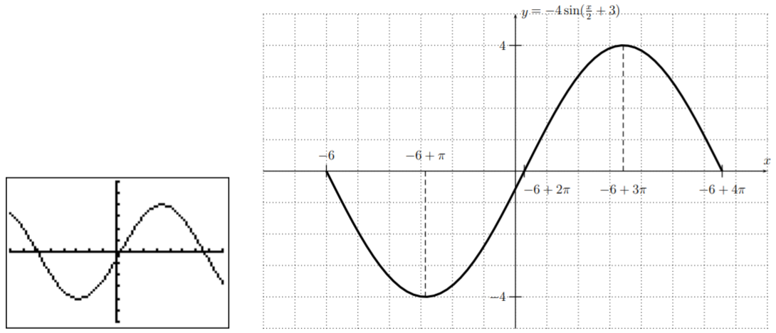
- \(f(x)=-4\cdot \sin\left(\dfrac{x}{2}+3\right)\)
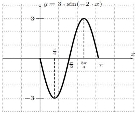
- \(f(x)=3 \sin(-2 x)\)
Solution
- The amplitude is \(|3|=3\), and since \(f(x)=3\cdot \sin(2\cdot x+0)\), it is \(b=2\) and \(c=0\), so that the period is \(\left|\dfrac{2\pi}{2}\right|=\pi\) and the phase-shift is \(\dfrac{-0}{2}=0\). This is also supported by graphing the function with the calculator; in particular the graph repeats after one full period, which is at \(\pi\approx 3.1\).
- For \(f(x)=-2\cos(\pi\cdot x)\), the amplitude is \(|-2|=2\), the period is \(\left|\dfrac{2\pi}{\pi}\right|=2\), and the phase-shift is \(0\). Note, that the first coefficient is negative, so that the \(\cos(x)\) has to be reflected about the \(x\)-axis. One full period is graphed below with a solid line (and the continuation of the graph is dashed). This graph is again supported by the graph and table as given by the calculator.
- The amplitude of \(f(x)=\cos(x-2)\) is \(1\), the period is \(2\pi\), and the phase-shift is \(\dfrac{-(-2)}{1}=2\). The graph over one period is displayed below.

The minimum of the function \(f\) in this period is given by taking the value in the middle of the interval \([2,2+2\pi]\), that is at \(2+\pi\). With this, the zeros are given by taking the value in the middle of the intervals \([2,2+\pi]\) and \([2+\pi,2+2\pi]\), which are at \(2+\dfrac{\pi}{2}\) and \(2+\dfrac{3\pi}{2}\).
- The function \(f(x)=\cos(2 x+\pi)\) has amplitude \(1\), period \(\dfrac{2\pi}{2}=\pi\), and phase-shift \(\dfrac{-\pi}{2}\). We may thus draw the graph over one period from \(\dfrac{-\pi}{2}\) to \(\dfrac{-\pi}{2}+\pi=\dfrac{\pi}{2}\); see graph on the left below. However, we may also graph the function over another full period, such as \([0,\pi]\) (see the graph on the right).

- The graph of \(f(x)=-4\cdot \sin\left(\dfrac{x}{2}+3\right)\) has an amplitude of \(|-4|=4\), a period of \(\dfrac{2\pi}{\frac{1}{2}}=4\pi\), and a phase shift of \(\dfrac{-3}{\frac{1}{2}}=-6\). Using this information, and confirming this with the calculator, we can draw one full period of the graph of \(f\).
- For \(f(x)=3\sin(-2x)\), we have an amplitude of \(3\), a period of \(\left|\dfrac{2\pi}{-2}\right|=\pi\) and a phase-shift of \(\dfrac{-0}{-2}=0\). Comparing this with example (a) above, we see that we have the same data as for the function \(y=3\sin(2x)\) from part (a). However, in this case, we have to draw the sine function over one period moving to the left, which means that the graph has to start the period as a decreasing function. This can also be seen by observing that the sine function is an odd function, that is equation \(\ref{EQ:sin-odd-cos-even}\), so that
\[f(x)=3\sin(-2x) = -3\sin(2x) \nonumber \]
The graph is therefore drawn as follows.