26.2: A.2 Graphing a function

Last updated
Save as PDF

Page ID: 54489

Thomas Tradler and Holly Carley
CUNY New York City College of Technology via New York City College of Technology at CUNY Academic Works

$ \newcommand{\vecs}[1]{\overset { \scriptstyle \rightharpoonup} {\mathbf{#1}} } $ $ \newcommand{\vecd}[1]{\overset{-\!-\!\rightharpoonup}{\vphantom{a}\smash {#1}}} $$\newcommand{\id}{\mathrm{id}}$ $ \newcommand{\Span}{\mathrm{span}}$ $ \newcommand{\kernel}{\mathrm{null}\,}$ $ \newcommand{\range}{\mathrm{range}\,}$ $ \newcommand{\RealPart}{\mathrm{Re}}$ $ \newcommand{\ImaginaryPart}{\mathrm{Im}}$ $ \newcommand{\Argument}{\mathrm{Arg}}$ $ \newcommand{\norm}[1]{\| #1 \|}$ $ \newcommand{\inner}[2]{\langle #1, #2 \rangle}$ $ \newcommand{\Span}{\mathrm{span}}$ $\newcommand{\id}{\mathrm{id}}$ $ \newcommand{\Span}{\mathrm{span}}$ $ \newcommand{\kernel}{\mathrm{null}\,}$ $ \newcommand{\range}{\mathrm{range}\,}$ $ \newcommand{\RealPart}{\mathrm{Re}}$ $ \newcommand{\ImaginaryPart}{\mathrm{Im}}$ $ \newcommand{\Argument}{\mathrm{Arg}}$ $ \newcommand{\norm}[1]{\| #1 \|}$ $ \newcommand{\inner}[2]{\langle #1, #2 \rangle}$ $ \newcommand{\Span}{\mathrm{span}}$$\newcommand{\AA}{\unicode[.8,0]{x212B}}$

The Y= screen

This is the screen that we will need to graph functions. It is seen by pressing $\boxed{y=}$.

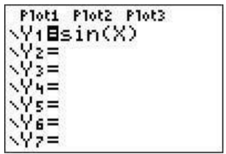
$clipboard_ee33d58ebdeb1dcb8fda2b4a81ceb3c43.png$

Press the $\boxed{y=}$ button. This brings you to the screen where you can enter functions that you want to graph. Let us suppose that you want to graph $y=\sin(x)$. You would first move the cursor (using the arrow keys) to ’Y1’ enter $\boxed{\sin}$$\boxed{\text{X,T,}\theta,n}$$\boxed{\text{enter}}$. The press $\boxed{\text{graph}}$. This will show a portion of the graph of the function (naturally, it can not generally show you the whole graph as this is often ’infinite’).

$clipboard_ece22e854f84d2fb6ec7df14916a99746.png$

Rescaling the graphing window

The graphing window is what determines what portion of the graph is seen. There are various reasons you may want to have a different window. For example, the standard view for graphing the sin function (as we will show in the next paragraph) the setting for the $y$-axis is too large and makes it difficult to see what is going on. We describe here a few using the example of $\sin(x)$ (in degree mode) and encourage experimenting.

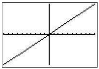
The standard window

This sets the $x$-axis from $-10$ to $10$ and the $y$-axis from $-10$ to $10$. To choose this view you must choose the standard window from the ’ZOOM’ screen by pressing $\boxed{\text{zoom}}$$\boxed{\text{6}}$. This is the window shown above.

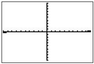
$clipboard_e5f95ee281e444a31b095437cb11ed786.png$

Notice that in this case you can’t really see what you want. Don’t worry, there are other zooming options!

Zoom fit

One easy way to ’choose’ an appropriate window is to ask the calculator to choose it using the ’zoom fit’ windows ($\boxed{\text{zoom}}$$\boxed{\text{0}}$). You can also press then press the down arrow until you arrive at the bottom of the list with is ’ZoomFit’.

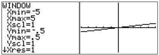
$clipboard_e7e7b4716ed59012c0a74fc8f9a3c564a.png$

Custom window

Maybe the zoom fit choice of the calculator isn’t what you wanted to see. Then you can choose your own window. Press the ($\boxed{\text{window}}$ key. Move the cursor to Xmin. This is the smallest number on the $x$-axis in your custom window. let’s say you want this to be $-5$. Then you press ($\boxed{\text{(-)}}$($\boxed{\text{5}}$. Then move the cursor to Xmax and enter your desired maximum, say, ($\boxed{\text{5}}$. You can also adjust the scale (where the marks on the $x$-axis are given) by setting Xscl equal to whatever is convenient. In this example we will set it to $1$. Now you can do the same for the y-axis with changing Ymin and Ymax to say, ($\boxed{\text{(-)}}$($\boxed{\cdot}$($\boxed{\text{5}}$ and ($\boxed{\cdot}$($\boxed{\text{5}}$, respectively. Press graph again and observe the window.

$clipboard_e36b76a5bafdf37cddd0147c9d75d539c.png$

Zooming in and out

You can zoom in and out also. Press the $\boxed{\text{zoom}}$$\boxed{\text{2}}$. You will now be looking at the graph. Move your cursor to what you want to be the center and press $\boxed{\text{enter}}$. You can zoom out as well.

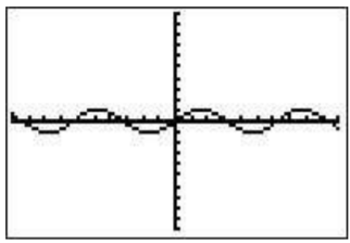
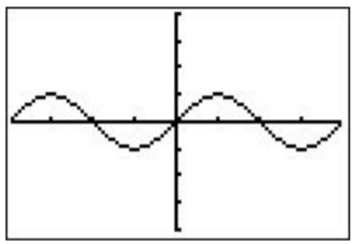
ZTrig

The best choice for our current Y1=$\sin($X$)$ function is ZTrig (press $\boxed{\text{zoom}}$$\boxed{\text{7}}$).

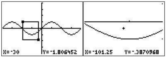
$clipboard_e0daaf878ecdce0a7edb1dda96a9493dd.png$

Zbox

You should experiment with ZBox, which is the first option on the zoom menu. You first move the cursor to where you want the upper left point of your box to be and press enter. Then you move the cursor to where you want your lower right corner to be and press enter. Our result is

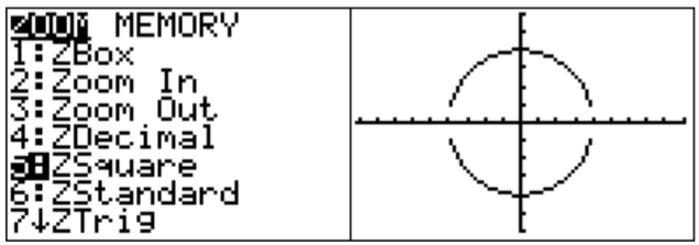
$clipboard_e0c6b37d133910890fae6c00814c9bd7d.png$

ZSquare

Finally, we point out another zoom option, the zoom square option, which scales the $x$- and $y$-axes to the same pixel size. To see the issue recall from Example 4.1.2, that the circle $x^2+y^2=16$ may be graphed by entering the functions $y=\pm\sqrt{16-x^2}$.

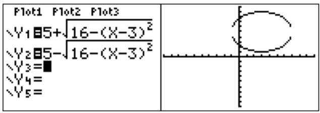
$clipboard_e251386cdfdff5b7c166471b959777438.png$

Note, that the obtained graph in the above window (with $-6\leq x\leq 6$ and $-6\leq y\leq 6$) looks more like an ellipse rather than a circle. To rectify this, we press $\boxed{\text{zoom}}$$\boxed{\text{5}}$, and obtain a graph which now does have the shape of a circle.

$clipboard_e84cce15f3562b73b35efe6d788bb2409.png$