Mathematics LibreTexts

1.6.9.3.8: Answers to exercises

  • Page ID
    32681
  • \( \newcommand{\vecs}[1]{\overset { \scriptstyle \rightharpoonup} {\mathbf{#1}} } \)

    \( \newcommand{\vecd}[1]{\overset{-\!-\!\rightharpoonup}{\vphantom{a}\smash {#1}}} \)

    \( \newcommand{\id}{\mathrm{id}}\) \( \newcommand{\Span}{\mathrm{span}}\)

    ( \newcommand{\kernel}{\mathrm{null}\,}\) \( \newcommand{\range}{\mathrm{range}\,}\)

    \( \newcommand{\RealPart}{\mathrm{Re}}\) \( \newcommand{\ImaginaryPart}{\mathrm{Im}}\)

    \( \newcommand{\Argument}{\mathrm{Arg}}\) \( \newcommand{\norm}[1]{\| #1 \|}\)

    \( \newcommand{\inner}[2]{\langle #1, #2 \rangle}\)

    \( \newcommand{\Span}{\mathrm{span}}\)

    \( \newcommand{\id}{\mathrm{id}}\)

    \( \newcommand{\Span}{\mathrm{span}}\)

    \( \newcommand{\kernel}{\mathrm{null}\,}\)

    \( \newcommand{\range}{\mathrm{range}\,}\)

    \( \newcommand{\RealPart}{\mathrm{Re}}\)

    \( \newcommand{\ImaginaryPart}{\mathrm{Im}}\)

    \( \newcommand{\Argument}{\mathrm{Arg}}\)

    \( \newcommand{\norm}[1]{\| #1 \|}\)

    \( \newcommand{\inner}[2]{\langle #1, #2 \rangle}\)

    \( \newcommand{\Span}{\mathrm{span}}\) \( \newcommand{\AA}{\unicode[.8,0]{x212B}}\)

    \( \newcommand{\vectorA}[1]{\vec{#1}}      % arrow\)

    \( \newcommand{\vectorAt}[1]{\vec{\text{#1}}}      % arrow\)

    \( \newcommand{\vectorB}[1]{\overset { \scriptstyle \rightharpoonup} {\mathbf{#1}} } \)

    \( \newcommand{\vectorC}[1]{\textbf{#1}} \)

    \( \newcommand{\vectorD}[1]{\overrightarrow{#1}} \)

    \( \newcommand{\vectorDt}[1]{\overrightarrow{\text{#1}}} \)

    \( \newcommand{\vectE}[1]{\overset{-\!-\!\rightharpoonup}{\vphantom{a}\smash{\mathbf {#1}}}} \)

    \( \newcommand{\vecs}[1]{\overset { \scriptstyle \rightharpoonup} {\mathbf{#1}} } \)

    \( \newcommand{\vecd}[1]{\overset{-\!-\!\rightharpoonup}{\vphantom{a}\smash {#1}}} \)

    \(\newcommand{\avec}{\mathbf a}\) \(\newcommand{\bvec}{\mathbf b}\) \(\newcommand{\cvec}{\mathbf c}\) \(\newcommand{\dvec}{\mathbf d}\) \(\newcommand{\dtil}{\widetilde{\mathbf d}}\) \(\newcommand{\evec}{\mathbf e}\) \(\newcommand{\fvec}{\mathbf f}\) \(\newcommand{\nvec}{\mathbf n}\) \(\newcommand{\pvec}{\mathbf p}\) \(\newcommand{\qvec}{\mathbf q}\) \(\newcommand{\svec}{\mathbf s}\) \(\newcommand{\tvec}{\mathbf t}\) \(\newcommand{\uvec}{\mathbf u}\) \(\newcommand{\vvec}{\mathbf v}\) \(\newcommand{\wvec}{\mathbf w}\) \(\newcommand{\xvec}{\mathbf x}\) \(\newcommand{\yvec}{\mathbf y}\) \(\newcommand{\zvec}{\mathbf z}\) \(\newcommand{\rvec}{\mathbf r}\) \(\newcommand{\mvec}{\mathbf m}\) \(\newcommand{\zerovec}{\mathbf 0}\) \(\newcommand{\onevec}{\mathbf 1}\) \(\newcommand{\real}{\mathbb R}\) \(\newcommand{\twovec}[2]{\left[\begin{array}{r}#1 \\ #2 \end{array}\right]}\) \(\newcommand{\ctwovec}[2]{\left[\begin{array}{c}#1 \\ #2 \end{array}\right]}\) \(\newcommand{\threevec}[3]{\left[\begin{array}{r}#1 \\ #2 \\ #3 \end{array}\right]}\) \(\newcommand{\cthreevec}[3]{\left[\begin{array}{c}#1 \\ #2 \\ #3 \end{array}\right]}\) \(\newcommand{\fourvec}[4]{\left[\begin{array}{r}#1 \\ #2 \\ #3 \\ #4 \end{array}\right]}\) \(\newcommand{\cfourvec}[4]{\left[\begin{array}{c}#1 \\ #2 \\ #3 \\ #4 \end{array}\right]}\) \(\newcommand{\fivevec}[5]{\left[\begin{array}{r}#1 \\ #2 \\ #3 \\ #4 \\ #5 \\ \end{array}\right]}\) \(\newcommand{\cfivevec}[5]{\left[\begin{array}{c}#1 \\ #2 \\ #3 \\ #4 \\ #5 \\ \end{array}\right]}\) \(\newcommand{\mattwo}[4]{\left[\begin{array}{rr}#1 \amp #2 \\ #3 \amp #4 \\ \end{array}\right]}\) \(\newcommand{\laspan}[1]{\text{Span}\{#1\}}\) \(\newcommand{\bcal}{\cal B}\) \(\newcommand{\ccal}{\cal C}\) \(\newcommand{\scal}{\cal S}\) \(\newcommand{\wcal}{\cal W}\) \(\newcommand{\ecal}{\cal E}\) \(\newcommand{\coords}[2]{\left\{#1\right\}_{#2}}\) \(\newcommand{\gray}[1]{\color{gray}{#1}}\) \(\newcommand{\lgray}[1]{\color{lightgray}{#1}}\) \(\newcommand{\rank}{\operatorname{rank}}\) \(\newcommand{\row}{\text{Row}}\) \(\newcommand{\col}{\text{Col}}\) \(\renewcommand{\row}{\text{Row}}\) \(\newcommand{\nul}{\text{Nul}}\) \(\newcommand{\var}{\text{Var}}\) \(\newcommand{\corr}{\text{corr}}\) \(\newcommand{\len}[1]{\left|#1\right|}\) \(\newcommand{\bbar}{\overline{\bvec}}\) \(\newcommand{\bhat}{\widehat{\bvec}}\) \(\newcommand{\bperp}{\bvec^\perp}\) \(\newcommand{\xhat}{\widehat{\xvec}}\) \(\newcommand{\vhat}{\widehat{\vvec}}\) \(\newcommand{\uhat}{\widehat{\uvec}}\) \(\newcommand{\what}{\widehat{\wvec}}\) \(\newcommand{\Sighat}{\widehat{\Sigma}}\) \(\newcommand{\lt}{<}\) \(\newcommand{\gt}{>}\) \(\newcommand{\amp}{&}\) \(\definecolor{fillinmathshade}{gray}{0.9}\)

    Answer to the sundew wetness question. Let us apply the approach we used for the leaf shape:

    Code \(\PageIndex{1}\) (R):

    leaf <- read.table("data/sundew.txt", h=TRUE, sep=";")
    wet <- ts(leaf$WET, frequency=36)
    str(wet)
    acf(wet)
    plot(stl(wet, s.window="periodic")$time.series)

    (Plots are not shown, please make them yourself.)

    There is some periodicity with 0.2 (5 hours) period. However, trend is likely absent.

    Answer to the dodder infestation question. Inspect the data, load and check:

    Code \(\PageIndex{2}\) (R):

    cu <- read.table("http://ashipunov.info/shipunov/open/cuscuta.txt",h=TRUE, sep="	")
    str(cu)
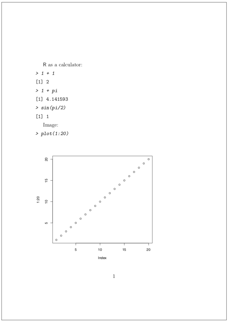
    Screen Shot 2019-02-01 at 10.29.29 PM.png Figure \(\PageIndex{1}\) The example of Sweave() report.

    (Note that two last columns are ranked. Consequently, only nonparametric methods are applicable here.)

    Then we need to select two hosts of question and drop unused levels:

    Code \(\PageIndex{3}\) (R):

    cu <- read.table("http://ashipunov.info/shipunov/open/cuscuta.txt",h=TRUE, sep="	")
    cu2 <- cu[cu$HOST %in% c("Alchemilla","Knautia"), ]
    cu2 <- droplevels(cu2)

    It is better to convert this to the short form:

    Code \(\PageIndex{4}\) (R):

    cu <- read.table("http://ashipunov.info/shipunov/open/cuscuta.txt",h=TRUE, sep="	")
    cu2 <- cu[cu$HOST %in% c("Alchemilla","Knautia"), ]
    cu2 <- droplevels(cu2)
    cu2.s <- split(cu2$DEGREE, cu2$HOST)

    No look on these samples graphically:

    Code \(\PageIndex{5}\) (R):

    cu <- read.table("http://ashipunov.info/shipunov/open/cuscuta.txt",h=TRUE, sep="	")
    cu2 <- cu[cu$HOST %in% c("Alchemilla","Knautia"), ]
    cu2 <- droplevels(cu2)
    cu2.s <- split(cu2$DEGREE, cu2$HOST)
    boxplot(cu2.s)

    There is a prominent difference. Now to numbers:

    Code \(\PageIndex{6}\) (R):

    cu <- read.table("http://ashipunov.info/shipunov/open/cuscuta.txt",h=TRUE, sep="	")
    cu2 <- cu[cu$HOST %in% c("Alchemilla","Knautia"), ]
    cu2 <- droplevels(cu2)
    cu2.s <- split(cu2$DEGREE, cu2$HOST)
    sapply(cu2.s, median)
    cliff.delta(cu2.s$Alchemilla, cu2.s$Knautia)
    wilcox.test(cu2.s$Alchemilla, cu2.s$Knautia)

    Interesting! Despite on the difference between medians and large effect size, Wilcoxon test failed to support it statistically. Why? Were shapes of distributions similar?

    Code \(\PageIndex{7}\) (R):

    cu <- read.table("http://ashipunov.info/shipunov/open/cuscuta.txt",h=TRUE, sep="	")
    cu2 <- cu[cu$HOST %in% c("Alchemilla","Knautia"), ]
    cu2 <- droplevels(cu2)
    cu2.s <- split(cu2$DEGREE, cu2$HOST)
    ansari.test(cu2.s$Alchemilla, cu2.s$Knautia)
    library(beeswarm)
    la <- layout(matrix(c(1, 3, 2, 3), ncol=2, byrow=TRUE))
    for (i in 1:2) hist(cu2.s[[i]], main=names(cu2.s)[i], xlab="", xlim=range(cu2.s))
    bxplot(cu2.s) ; beeswarm(cu2.s, cex=1.2, add=TRUE)

    (Please note how to make complex layout with layout() command. This commands takes matrix as argument, and then simply place plot number something to the position where this number occurs in the matrix. After layout was created, you can check it with command layout.show(la).)
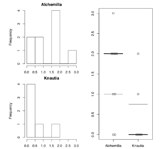
    Screen Shot 2019-02-01 at 10.28.10 PM.png Figure \(\PageIndex{2}\) Histograms of two sample distributions, plus beswarm plot with boxplot lines.

    As both Ansari-Bradley test and plots suggest, distributions are really different (Figure \(\PageIndex{2}\)). One workaround is to use robust rank order test which is not so sensitive to the differences in variation:

    Code \(\PageIndex{8}\) (R):

    cu <- read.table("http://ashipunov.info/shipunov/open/cuscuta.txt",h=TRUE, sep="	")
    cu2 <- cu[cu$HOST %in% c("Alchemilla","Knautia"), ]
    cu2 <- droplevels(cu2)
    cu2.s <- split(cu2$DEGREE, cu2$HOST)
    Rro.test(cu2.s$Alchemilla, cu2.s$Knautia) # asmisc.r

    This test found the significance.

    Now we will try to bootstrap the difference between medians:

    Code \(\PageIndex{9}\) (R):

    cu <- read.table("http://ashipunov.info/shipunov/open/cuscuta.txt",h=TRUE, sep="	")
    cu2 <- cu[cu$HOST %in% c("Alchemilla","Knautia"), ]
    cu2 <- droplevels(cu2)
    cu2.s <- split(cu2$DEGREE, cu2$HOST)
    library(boot)
    meddif.b <- function (data, ind) { d <- data[ind]; median(d[cu2$HOST == "Alchemilla"]) - median(d[cu2$HOST == "Knautia"]) }
    meddif.boot <- boot(data=cu2$DEGREE, statistic=meddif.b, strata=cu2$HOST, R=999)
    boot.ci(meddif.boot, type="bca")

    (Please note how strata was applied to avoid mixing of two different hosts.)

    This is not dissimilar to what we saw above in the effect size output: large difference but 0 included. This could be described as “prominent but unstable” difference.

    That was not asked in assignment but how to analyze whole data in case of so different shapes of distributions. One possibility is the Kruskal test with Monte-Carlo replications. By default, it makes 1000 tries:

    Code \(\PageIndex{10}\) (R):

    cu <- read.table("http://ashipunov.info/shipunov/open/cuscuta.txt",h=TRUE, sep="	")
    library(coin)
    kruskal_test(DEGREE ~ HOST, data=cu, distribution=approximate())

    There is no overall significance. It is not a surprise, ANOVA-like tests could sometimes contradict with individual or pairwise.

    Another possibility is a post hoc robust rank order test:

    Code \(\PageIndex{11}\) (R):

    cu <- read.table("http://ashipunov.info/shipunov/open/cuscuta.txt",h=TRUE, sep="	")
    pairwise.Rro.test(cu$DEGREE, cu$HOST) # asmisc.r

    Now it found some significant differences but did not reveal it for our marginal, unstable case of Alchemilla and Knautia.


    1.6.9.3.8: Answers to exercises is shared under a not declared license and was authored, remixed, and/or curated by LibreTexts.

    • Was this article helpful?