3.1: Introducing the Derivative

Learning Objectives

• Recognize the meaning of the tangent to a curve at a point.
• Calculate the slope of a tangent line.
• Identify the derivative as the limit of a difference quotient.
• Calculate the derivative of a given function at a point.
• Describe the velocity as a rate of change.
• Explain the difference between average velocity and instantaneous velocity.
• Estimate the derivative from a table of values.
• Define the derivative function of a given function.
• Graph a derivative function from the graph of a given function.
• State the connection between derivatives and continuity.
• Describe three conditions for when a function does not have a derivative.
• Explain the meaning of a higher-order derivative.

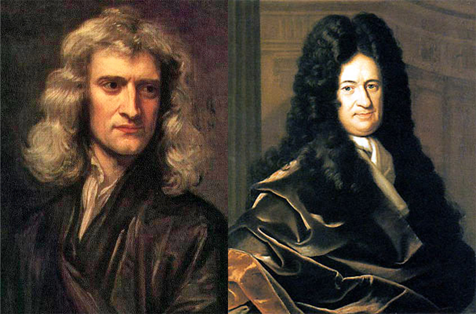
Now that we have both a conceptual understanding of a limit and the practical ability to compute limits, we have established the foundation for our study of calculus, the branch of mathematics in which we compute derivatives and integrals. Most mathematicians and historians agree that calculus was developed independently by the Englishman Isaac Newton (1643–1727) and the German Gottfried Leibniz (1646–1716), whose images appear in Figure \(\PageIndex{1}\). When we credit Newton and Leibniz with developing calculus, we are really referring to the fact that Newton and Leibniz were the first to understand the relationship between the derivative and the integral. Both mathematicians benefited from the work of predecessors, such as Barrow, Fermat, and Cavalieri. The initial relationship between the two mathematicians appears to have been amicable; however, in later years a bitter controversy erupted over whose work took precedence. Although it seems likely that Newton did, indeed, arrive at the ideas behind calculus first, we are indebted to Leibniz for the notation that we commonly use today.

Figure \(\PageIndex{1}\): Newton and Leibniz are credited with developing calculus independently.

Tangent Lines

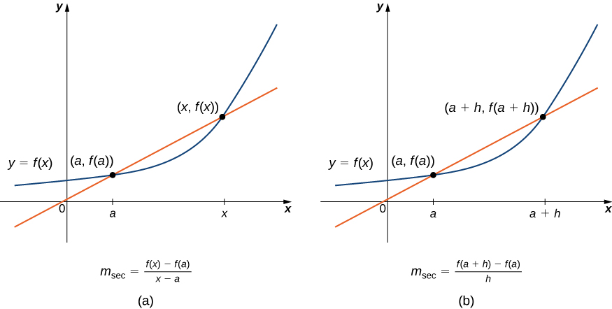
We begin our study of calculus by revisiting the notion of secant lines and tangent lines. Recall that we used the slope of a secant line to a function at a point \((a,f(a))\) to estimate the rate of change, or the rate at which one variable changes in relation to another variable. We can obtain the slope of the secant by choosing a value of x near a and drawing a line through the points \((a,f(a))\) and \((x,f(x))\), as shown in Figure \(\PageIndex{2}\). The slope of this line is given by an equation in the form of a difference quotient:

\[m_{sec}=\frac{f(x)−f(a)}{x−a} \nonumber \]

We can also calculate the slope of a secant line to a function at a value a by using this equation and replacing \(x\) with \(a+h\), where \(h\) is a value close to a. We can then calculate the slope of the line through the points \((a,f(a))\) and \((a+h,f(a+h))\). In this case, we find the secant line has a slope given by the following difference quotient with increment \(h\):

\[m_{sec}=\frac{f(a+h)−f(a)}{a+h−a}=\frac{f(a+h)−f(a)}{h} \nonumber \]

Definition: Difference Quotient

Let \(f\) be a function defined on an interval \(I\) containing \(a\). If \(x≠a\) is in \(I\), then

\[Q=\frac{f(x)−f(a)}{x−a}\]

is a difference quotient.

Also, if \(h≠0\) is chosen so that \(a+h\) is in \(I\), then

\[Q=\frac{f(a+h)−f(a)}{h}\]

is a difference quotient with increment \(h\).

These two expressions for calculating the slope of a secant line are illustrated in Figure \(\PageIndex{2}\). We will see that each of these two methods for finding the slope of a secant line is of value. Depending on the setting, we can choose one or the other. The primary consideration in our choice usually depends on ease of calculation.

Figure \(\PageIndex{2}\): We can calculate the slope of a secant line in either of two ways.

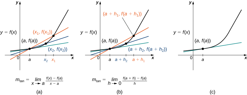
In Figure \(\PageIndex{3a}\) we see that, as the values of \(x\) approach \(a\), the slopes of the secant lines provide better estimates of the rate of change of the function at \(a\). Furthermore, the secant lines themselves approach the tangent line to the function at \(a\), which represents the limit of the secant lines. Similarly, Figure \(\PageIndex{3b}\) shows that as the values of \(h\) get closer to \(0\), the secant lines also approach the tangent line. The slope of the tangent line at \(a\) is the rate of change of the function at \(a\), as shown in Figure \(\PageIndex{3c}\).

Figure \(\PageIndex{3}\): The secant lines approach the tangent line (shown in green) as the second point approaches the first.

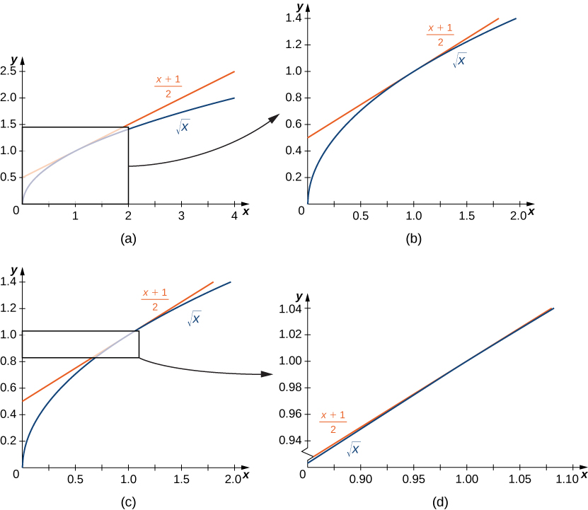
In Figure \(\PageIndex{4}\) we show the graph of \(f(x)=\sqrt{x}\) and its tangent line at \((1,1)\) in a series of tighter intervals about \(x=1\). As the intervals become narrower, the graph of the function and its tangent line appear to coincide, making the values on the tangent line a good approximation to the values of the function for choices of \(x\) close to \(1\). In fact, the graph of \(f(x)\) itself appears to be locally linear in the immediate vicinity of \(x=1\).

Figure \(\PageIndex{4}\): For values of \(x\) close to \(1\), the graph of \(f(x)=\sqrt{x}\) and its tangent line appear to coincide.

Formally we may define the tangent line to the graph of a function as follows.

Definition: Tangent Line

Let \(f(x)\) be a function defined in an open interval containing \(a\). The tangent line to \(f(x)\) at \(a\) is the line passing through the point \((a,f(a))\) having slope

\[m_{tan}=\lim_{x→a}\frac{f(x)−f(a)}{x−a} \label{tanline1}\]

provided this limit exists.

Equivalently, we may define the tangent line to \(f(x)\) at \(a\) to be the line passing through the point \((a,f(a))\) having slope

\[m_{tan}=\lim_{h→0}\frac{f(a+h)−f(a)}{h} \label{tanline2}\]

provided this limit exists.

Just as we have used two different expressions to define the slope of a secant line, we use two different forms to define the slope of the tangent line. In this text we use both forms of the definition. As before, the choice of definition will depend on the setting. Now that we have formally defined a tangent line to a function at a point, we can use this definition to find equations of tangent lines.

Example \(\PageIndex{1}\): Finding a Tangent Line

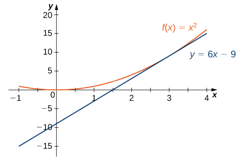
Find the equation of the line tangent to the graph of \(f(x)=x^2\) at \(x=3.\)

Solution

First find the slope of the tangent line. In this example, use Equation \ref{tanline1}.

\(\displaystyle \begin{align*} m_{tan}&=\lim_{x→3}\frac{f(x)−f(3)}{x−3} & & \text{Apply the definition.}\\[4pt]
&=\lim_{x→3}\frac{x^2−9}{x−3} & & \text{Substitute }f(x)=x^2\text{ and }f(3)=9\\[4pt]
&=\lim_{x→3}\frac{(x−3)(x+3)}{x−3} =\lim_{x→3}(x+3)=6 & & \text{Factor the numerator to evaluate the limit.}\end{align*}\)

Next, find a point on the tangent line. Since the line is tangent to the graph of \(f(x)\) at \(x=3\), it passes through the point \((3,f(3))\). We have \(f(3)=9\), so the tangent line passes through the point \((3,9)\).

Using the point-slope equation of the line with the slope \(m=6\) and the point \((3,9)\), we obtain the line \(y−9=6(x−3)\). Simplifying, we have \(y=6x−9\). The graph of \(f(x)=x^2\) and its tangent line at \(3\) are shown in Figure \(\PageIndex{5}\).

Figure \(\PageIndex{5}\): The tangent line to \(f(x)\) at \(x=3\).

Example \(\PageIndex{2}\): The Slope of a Tangent Line Revisited

Use Equation \ref{tanline2} to find the slope of the line tangent to the graph of \(f(x)=x^2\) at \(x=3\).

Solution

The steps are very similar to Example \(\PageIndex{2}\). See Equation \ref{tanline2} for the definition.

\(\begin{align*} m_{tan}&=\lim_{h→0}\frac{f(3+h)−f(3)}{h} & & \text{Apply the definition.}\\[4pt]
&=\lim_{h→0}\frac{(3+h)^2−9}{h} & & \text{Substitute }f(3+h)=(3+h)^2\text{ and }f(3)=9\\[4pt]
&=\lim_{h→0}\frac{9+6h+h^2−9}{h} & & \text{Expand and simplify to evaluate the limit.}\\[4pt]
&=\lim_{h→0}\frac{h(6+h)}{h}=\lim_{h→0}(6+h)=6 \end{align*}\)

We obtained the same value for the slope of the tangent line by using the other definition, demonstrating that the formulas can be interchanged.

Example \(\PageIndex{3}\): Finding the Equation of a Tangent Line

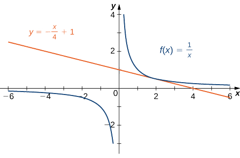
Find the equation of the line tangent to the graph of \(f(x)=1/x\) at \(x=2\).

Solution

We can use Equation \ref{tanline1}, but as we have seen, the results are the same if we use Equation \ref{tanline2}.

\(\displaystyle \begin{align*} m_{tan}&=\lim_{x→2}\frac{f(x)−f(2)}{x−2} & & \text{Apply the definition.}\\[4pt]
&=\lim_{x→2}\frac{\frac{1}{x}−\frac{1}{2}}{x−2} & & \text{Substitute }f(x)=\frac{1}{x}\text{ and }f(2)=\frac{1}{2}\\[4pt]
&=\lim_{x→2}\frac{\frac{1}{x}−\frac{1}{2}}{x−2}⋅\frac{2x}{2x} & & \text{Multiply numerator and denominator by }2x\text{ to simplify fractions.}\\[4pt]
&=\lim_{x→2}\frac{(2−x)}{(x−2)(2x)} & & \text{Simplify.}\\[4pt]
&=\lim_{x→2}\frac{−1}{2x} & & \text{Simplify using }\frac{2−x}{x−2}=−1,\text{ for }x≠2.\\[4pt]
&=−\frac{1}{4} & & \text{Evaluate the limit.}\end{align*}\)

We now know that the slope of the tangent line is \(−\frac{1}{4}\). To find the equation of the tangent line, we also need a point on the line. We know that \(f(2)=\frac{1}{2}\). Since the tangent line passes through the point \((2,\frac{1}{2})\) we can use the point-slope equation of a line to find the equation of the tangent line. Thus the tangent line has the equation \(y=−\frac{1}{4}x+1\). The graphs of \(f(x)=\frac{1}{x}\) and \(y=−\frac{1}{4}x+1\) are shown in Figure \(\PageIndex{6}\).

Figure \(\PageIndex{6}\):The line is tangent to \(f(x)\) at \(x=2\).

Exercise \(\PageIndex{1}\)

Find the slope of the line tangent to the graph of \(f(x)=\sqrt{x}\) at \(x=4\).

Hint

Use either Equation \ref{tanline1} or Equation \ref{tanline2}. Multiply the numerator and the denominator by a conjugate.

Answer

\(\frac{1}{4}\)

The Derivative of a Function at a Point

The type of limit we compute in order to find the slope of the line tangent to a function at a point occurs in many applications across many disciplines. These applications include velocity and acceleration in physics, marginal profit functions in business, and growth rates in biology. This limit occurs so frequently that we give this value a special name: the derivative. The process of finding a derivative is called differentiation.

Definition: Derivative

Let \(f(x)\) be a function defined in an open interval containing \(a\). The derivative of the function \(f(x)\) at \(a\), denoted by \(f′(a)\), is defined by

\[f′(a)=\lim_{x→a}\frac{f(x)−f(a)}{x−a} \label{der1}\]

provided this limit exists.

Alternatively, we may also define the derivative of \(f(x)\) at \(a\) as

\[f′(a)=\lim_{h→0}\frac{f(a+h)−f(a)}{h}. \label{der2}\]

Example \(\PageIndex{4}\): Estimating a Derivative

For \(f(x)=x^2\), use a table to estimate \(f′(3)\) using Equation \ref{der1}.

Solution

Create a table using values of \(x\) just below \(3\) and just above \(3\).

\(x\)	\(\dfrac{x^2−9}{x−3}\)
2.9	5.9
2.99	5.99
2.999	5.999
3.001	6.001
3.01	6.01
3.1	6.1

After examining the table, we see that a good estimate is \(f′(3)=6\).

Exercise \(\PageIndex{2}\)

For \(f(x)=x^2\), use a table to estimate \(f′(3)\) using Equation \ref{der2}.

Hint

Evaluate \(\dfrac{(x+h)−x^2}{h}\) at \(h=−0.1,\,−0.01,\,−0.001,\,0.001,\,0.01,\,0.1\)

Answer

6

Example \(\PageIndex{6}\): Finding a Derivative

For \(f(x)=3x^2−4x+1\), find \(f′(2)\) by using Equation \ref{der1}.

Solution

Substitute the given function and value directly into the equation.

\(\displaystyle \begin{align*} f′(x)&=\lim_{x→2}\frac{f(x)−f(2)}{x−2} & & \text{Apply the definition.}\\[4pt]
&=\lim_{x→2}\frac{(3x^2−4x+1)−5}{x−2} & & \text{Substitute }f(x)=3x^2−4x+1\text{ and }f(2)=5.\\[4pt]
&=\lim_{x→2}\frac{(x−2)(3x+2)}{x−2} & & \text{Simplify and factor the numerator.}\\[4pt]
&=\lim_{x→2}(3x+2) & & \text{Cancel the common factor.}\\[4pt]
&=8 & & \text{Evaluate the limit.}\end{align*}\)

Example \(\PageIndex{7}\): Revisiting the Derivative

For \(f(x)=3x^2−4x+1\), find \(f′(2)\) by using Equation \ref{der2}.

Solution

Using this equation, we can substitute two values of the function into the equation, and we should get the same value as in Example \(\PageIndex{6}\).

\(\displaystyle \begin{align*} f′(2)&=\lim_{h→0}\frac{f(2+h)−f(2)}{h} & & \text{Apply the definition.}\\[4pt]
&=\lim_{h→0}\frac{(3(2+h)^2−4(2+h)+1)−5}{h} & & \text{Substitute }f(2)=5\text{ and }f(2+h)=3(2+h)^2−4(2+h)+1.\\[4pt]
&=\lim_{h→0}\frac{3(4+4h+h^2)-8-4h+1-5}{h} & & \text{Expand the numerator.}\\[4pt]
&=\lim_{h→0}\frac{12+12h+3h^2-12-4h}{h} & & \text{Distribute and begin simplifying the numerator.}\\[4pt]
&=\lim_{h→0}\frac{3h^2+8h}{h} & & \text{Finish simplifying the numerator.}\\[4pt]
&=\lim_{h→0}\frac{h(3h+8)}{h} & & \text{Factor the numerator.}\\[4pt]
&=\lim_{h→0}(3h+8) & & \text{Cancel the common factor.}\\[4pt]
&=8 & & \text{Evaluate the limit.} \end{align*} \)

The results are the same whether we use Equation \ref{der1} or Equation \ref{der2}.

Exercise \(\PageIndex{4}\)

For \(f(x)=x^2+3x+2\), find \(f′(1)\).

Hint

Use either Equation \ref{der1}, Equation \ref{der2}, or try both.

Answer

\(f′(1)=5\)

Velocities and Rates of Change

Now that we can evaluate a derivative, we can use it in velocity applications. Recall that if \(s(t)\) is the position of an object moving along a coordinate axis, the average velocity of the object over a time interval \([a,t]\) if \(t>a\) or \([t,a]\) if \(t<a\) is given by the difference quotient

\[v_{ave}=\frac{s(t)−s(a)}{t−a}. \label{avgvel}\]

As the values of \(t\) approach \(a\), the values of \(v_{ave}\) approach the value we call the instantaneous velocity at \(a\). That is, instantaneous velocity at \(a\), denoted \(v(a)\), is given by

\[v(a)=s′(a)=\lim_{t→a}\frac{s(t)−s(a)}{t−a}. \label{instvel}\]

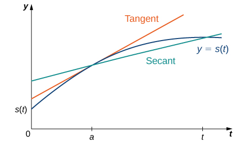
To better understand the relationship between average velocity and instantaneous velocity, see Figure \(\PageIndex{7}\). In this figure, the slope of the tangent line (shown in red) is the instantaneous velocity of the object at time \(t=a\) whose position at time \(t\) is given by the function \(s(t)\). The slope of the secant line (shown in green) is the average velocity of the object over the time interval \([a,t]\).

Figure \(\PageIndex{7}\): The slope of the secant line is the average velocity over the interval \([a,t]\). The slope of the tangent line is the instantaneous velocity.

We can use Equation \ref{instvel} to calculate the instantaneous velocity, or we can estimate the velocity of a moving object by using a table of values. We can then confirm the estimate by using Equation \ref{avgvel}.

Example \(\PageIndex{8}\): Estimating Velocity

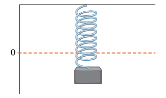
A lead weight on a spring is oscillating up and down. Its position at time \(t\) with respect to a fixed horizontal line is given by \(s(t)=\sin t\) (Figure \(\PageIndex{8}\)). Use a table of values to estimate \(v(0)\). Check the estimate by using Equation \ref{instvel}.

Figure \(\PageIndex{8}\): A lead weight suspended from a spring in vertical oscillatory motion.

Solution

We can estimate the instantaneous velocity at \(t=0\) by computing a table of average velocities using values of \(t\) approaching \(0\), as shown in Table \(\PageIndex{2}\).

Table \(\PageIndex{2}\): Average velocities using values of \(t\) approaching 0

\(t\)	\(\frac{\sin t−\sin 0}{t−0}=\frac{\sin t}{t}\)
−0.1	0.998334166
−0.01	0.9999833333
−0.001	0.999999833
0.001	0.999999833
0.01	0.9999833333
0.1	0.998334166

From the table we see that the average velocity over the time interval \([−0.1,0]\) is \(0.998334166\), the average velocity over the time interval \([−0.01,0]\) is \(0.9999833333\), and so forth. Using this table of values, it appears that a good estimate is \(v(0)=1\).

By using Equation \ref{instvel}, we can see that

\[v(0)=s′(0)=\lim_{t→0}\frac{\sin t−\sin 0}{t−0}=\lim_{t→0}\frac{\sin t}{t}=1. \nonumber\]

Thus, in fact, \(v(0)=1\).

Exercise \(\PageIndex{5}\)

A rock is dropped from a height of \(64\) feet. Its height above ground at time \(t\) seconds later is given by \(s(t)=−16t^2+64,\;0≤t≤2\). Find its instantaneous velocity \(1\) second after it is dropped, using Equation \ref{instvel}.

Hint

\(v(t)=s′(t)\). Follow the earlier examples of the derivative using Equation \ref{instvel}.

Answer

−32 ft/s

As we have seen throughout this section, the slope of a tangent line to a function and instantaneous velocity are related concepts. Each is calculated by computing a derivative and each measures the instantaneous rate of change of a function, or the rate of change of a function at any point along the function.

Definition: Instantaneous Rate of Change

The instantaneous rate of change of a function \(f(x)\) at a value \(a\) is its derivative \(f′(a)\).

Example \(\PageIndex{9}\): Chapter Opener: Estimating Rate of Change of Velocity

Reaching a top speed of \(270.49\) mph, the Hennessey Venom GT is one of the fastest cars in the world. In tests it went from \(0\) to \(60\) mph in \(3.05\) seconds, from \(0\) to \(100\) mph in \(5.88\) seconds, from \(0\) to \(200\) mph in \(14.51\) seconds, and from \(0\) to \(229.9\) mph in \(19.96\) seconds. Use this data to draw a conclusion about the rate of change of velocity (that is, its acceleration) as it approaches \(229.9\) mph. Does the rate at which the car is accelerating appear to be increasing, decreasing, or constant?

Figure \(\PageIndex{9}\): (credit: modification of work by Codex41, Flickr)

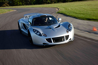
Solution: First observe that \(60\) mph = \(88\) ft/s, \(100\) mph ≈\(146.67\) ft/s, \(200\) mph ≈\(293.33\) ft/s, and \(229.9\) mph ≈\(337.19\) ft/s. We can summarize the information in a table.

Table \(\PageIndex{3}\): \(v(t)\) at different values of \(t\)

\(t\)	\(v(t)\)
0	0
3.05	88
5.88	147.67
14.51	293.33
19.96	337.19

Now compute the average acceleration of the car in feet per second on intervals of the form \([t,19.96]\) as \(t\) approaches \(19.96\), as shown in the following table.

Average acceleration

\(t\)	\(\dfrac{v(t)−v(19.96)}{t−19.96}=\dfrac{v(t)−337.19}{t−19.96}\)
0.0	16.89
3.05	14.74
5.88	13.46
14.51	8.05

The rate at which the car is accelerating is decreasing as its velocity approaches \(229.9\) mph (\(337.19\) ft/s).

Example \(\PageIndex{10}\): Rate of Change of Temperature

A homeowner sets the thermostat so that the temperature in the house begins to drop from \(70°F\) at \(9\) p.m., reaches a low of \(60°\) during the night, and rises back to \(70°\) by \(7\) a.m. the next morning. Suppose that the temperature in the house is given by \(T(t)=0.4t^2−4t+70\) for \(0≤t≤10\), where \(t\) is the number of hours past \(9\) p.m. Find the instantaneous rate of change of the temperature at midnight.

Solution

Since midnight is \(3\) hours past \(9\) p.m., we want to compute \(T′(3)\). Refer to Equation \ref{der1}.

\(\displaystyle \begin{align*} T′(3)&=\lim_{t→3}\frac{T(t)−T(3)}{t−3} & & \text{Apply the definition.}\\[4pt]
&=\lim_{t→3}\frac{0.4t^2−4t+70−61.6}{t−3} & & \text{Substitute }T(t)=0.4t^2−4t+70\text{ and }T(3)=61.6.\\[4pt]
&=\lim_{t→3}\frac{0.4t^2−4t+8.4}{t−3} & & \text{Simplify.}\\[4pt]
&=\lim_{t→3}\frac{0.4(t−3)(t−7)}{t−3}\\[4pt]
&=\lim_{t→3}0.4(t−7) & & \text{Cancel.}\\[4pt]
&=−1.6 & & \text{Evaluate the limit.} \end{align*}\)

The instantaneous rate of change of the temperature at midnight is \(−1.6°F\) per hour.

Example \(\PageIndex{11}\): Rate of Change of Profit

A toy company can sell \(x\) electronic gaming systems at a price of \(p=−0.01x+400\) dollars per gaming system. The cost of manufacturing \(x\) systems is given by \(C(x)=100x+10,000\) dollars. Find the rate of change of profit when \(10,000\) games are produced. Should the toy company increase or decrease production?

Solution

The profit \(P(x)\) earned by producing \(x\) gaming systems is \(R(x)−C(x)\), where \(R(x)\) is the revenue obtained from the sale of \(x\) games. Since the company can sell \(x\) games at \(p=−0.01x+400\) per game,

\(R(x)=xp=x(−0.01x+400)=−0.01x^2+400x\).

Consequently,

\(P(x)=−0.01x^2+300x−10,000\).

Therefore, evaluating the rate of change of profit gives

\(\displaystyle \begin{align*} P′(10000)&=\lim_{x→10000}\frac{P(x)−P(10000)}{x−10000}\\[4pt]
&=\lim_{x→10000}\frac{−0.01x^2+300x−10000−1990000}{x−10000}\\[4pt]
&=\lim_{x→10000}\frac{−0.01x^2+300x−2000000}{x−10000}\\[4pt]
&=100 \end{align*}\).

Since the rate of change of profit \(P′(10,000)>0\) and \(P(10,000)>0\), the company should increase production.

Exercise \(\PageIndex{6}\)

A coffee shop determines that the daily profit on scones obtained by charging s dollars per scone is \(P(s)=−20s^2+150s−10\). The coffee shop currently charges \($3.25\) per scone. Find \(P′(3.25)\), the rate of change of profit when the price is \($3.25\) and decide whether or not the coffee shop should consider raising or lowering its prices on scones.

Hint

Use Example \(\PageIndex{11}\) for a guide.

Answer

\(P′(3.25)=20>0\); raise prices

As we have seen, the derivative of a function at a given point gives us the rate of change or slope of the tangent line to the function at that point. If we differentiate a position function at a given time, we obtain the velocity at that time. It seems reasonable to conclude that knowing the derivative of the function at every point would produce valuable information about the behavior of the function. However, the process of finding the derivative at even a handful of values using the techniques of the preceding section would quickly become quite tedious. In this section we define the derivative function and learn a process for finding it.

Derivative Functions

The derivative function gives the derivative of a function at each point in the domain of the original function for which the derivative is defined. We can formally define a derivative function as follows.

Definition: Derivative Function

Let \(f\) be a function. The derivative function, denoted by \(f'\), is the function whose domain consists of those values of \(x\) such that the following limit exists:

\[f'(x)=\lim_{h→0}\frac{f(x+h)−f(x)}{h}. \label{derdef}\]

A function \(f(x)\) is said to be differentiable at \(a\) if \(f'(a)\) exists. More generally, a function is said to be differentiable on \(S\) if it is differentiable at every point in an open set \(S\), and a differentiable function is one in which \(f'(x)\) exists on its domain.

In the next few examples we use Equation \ref{derdef} to find the derivative of a function.

Example \(\PageIndex{1}\): Finding the Derivative of a Square-Root Function

Find the derivative of \(f(x)=\sqrt{x}\).

Solution

Start directly with the definition of the derivative function.

Substitute \(f(x+h)=\sqrt{x+h}\) and \(f(x)=\sqrt{x}\) into \(f'(x)= \displaystyle \lim_{h→0}\frac{f(x+h)−f(x)}{h}\).

\(f'(x)=\displaystyle \lim_{h→0}\frac{\sqrt{x+h}−\sqrt{x}}{h}\)
\(=\displaystyle\lim_{h→0}\frac{\sqrt{x+h}−\sqrt{x}}{h}⋅\frac{\sqrt{x+h}+\sqrt{x}}{\sqrt{x+h}+\sqrt{x}}\)	Multiply numerator and denominator by \(\sqrt{x+h}+\sqrt{x}\) without distributing in the denominator.
\(=\displaystyle\lim_{h→0}\frac{h}{h\left(\sqrt{x+h}+\sqrt{x}\right)}\)	Multiply the numerators and simplify.
\(=\displaystyle\lim_{h→0}\frac{1}{\left(\sqrt{x+h}+\sqrt{x}\right)}\)	Cancel the \(h\).
\(=\dfrac{1}{2\sqrt{x}}\)	Evaluate the limit

Example \(\PageIndex{2}\): Finding the Derivative of a Quadratic Function

Find the derivative of the function \(f(x)=x^2−2x\).

Solution

Follow the same procedure here, but without having to multiply by the conjugate.

Substitute \(f(x+h)=(x+h)^2−2(x+h)\) and \(f(x)=x^2−2x\) into \(f'(x)= \displaystyle \lim_{h→0}\frac{f(x+h)−f(x)}{h}.\)

\(f'(x)=\displaystyle\lim_{h→0}\frac{((x+h)^2−2(x+h))−(x^2−2x)}{h}\)
\(=\displaystyle\lim_{h→0}\frac{x^2+2xh+h^2−2x−2h−x^2+2x}{h}\)	Expand \((x+h)^2−2(x+h)\).
\(=\displaystyle\lim_{h→0}\frac{2xh−2h+h^2}{h}\)	Simplify
\(=\displaystyle\lim_{h→0}\frac{h(2x−2+h)}{h}\)	Factor out \(h\) from the numerator
\(=\displaystyle\lim_{h→0}(2x−2+h)\)	Cancel the common factor of \(h\)
\(=2x−2\)	Evaluate the limit

Exercise \(\PageIndex{1}\)

Find the derivative of \(f(x)=x^2\).

Hint

Use Equation \ref{derdef} and follow the example.

Answer

\(f'(x)=2x\)

We use a variety of different notations to express the derivative of a function. In Example we showed that if \(f(x)=x^2−2x\), then \(f'(x)=2x−2\). If we had expressed this function in the form \(y=x^2−2x\), we could have expressed the derivative as \(y′=2x−2\) or \(\dfrac{dy}{dx}=2x−2\). We could have conveyed the same information by writing \(\dfrac{d}{dx}\left(x^2−2x\right)=2x−2\). Thus, for the function \(y=f(x)\), each of the following notations represents the derivative of \(f(x)\):

\(f'(x), \quad \dfrac{dy}{dx}, \quad y′,\quad \dfrac{d}{dx}\big(f(x)\big)\).

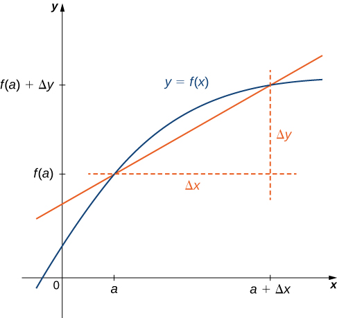
In place of \(f'(a)\) we may also use \(\dfrac{dy}{dx}\Big|_{x=a}\). Use of the \(\dfrac{dy}{dx}\) notation (called Leibniz notation) is quite common in engineering and physics. To understand this notation better, recall that the derivative of a function at a point is the limit of the slopes of secant lines as the secant lines approach the tangent line. The slopes of these secant lines are often expressed in the form \(\dfrac{Δy}{Δx}\) where \(Δy\) is the difference in the \(y\) values corresponding to the difference in the \(x\) values, which are expressed as \(Δx\) (Figure \(\PageIndex{1}\)). Thus the derivative, which can be thought of as the instantaneous rate of change of \(y\) with respect to \(x\), is expressed as

\(\displaystyle \frac{dy}{dx}= \lim_{Δx→0}\frac{Δy}{Δx}\).

Figure \(\PageIndex{1}\): The derivative is expressed as \(\dfrac{dy}{dx}=\displaystyle\lim_{Δx→0}\frac{Δy}{Δx}\).

Graphing a Derivative

We have already discussed how to graph a function, so given the equation of a function or the equation of a derivative function, we could graph it. Given both, we would expect to see a correspondence between the graphs of these two functions, since \(f'(x)\) gives the rate of change of a function \(f(x)\) (or slope of the tangent line to \(f(x)\)).

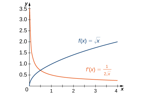
In Example \(\PageIndex{1}\), we found that for \(f(x)=\sqrt{x}\), \(f'(x)=\frac{1}{2\sqrt{x}}\). If we graph these functions on the same axes, as in Figure \(\PageIndex{2}\), we can use the graphs to understand the relationship between these two functions. First, we notice that \(f(x)\) is increasing over its entire domain, which means that the slopes of its tangent lines at all points are positive. Consequently, we expect \(f'(x)>0\) for all values of x in its domain. Furthermore, as \(x\) increases, the slopes of the tangent lines to \(f(x)\) are decreasing and we expect to see a corresponding decrease in \(f'(x)\). We also observe that \(f(0)\) is undefined and that \(\displaystyle \lim_{x→0^+}f'(x)=+∞\), corresponding to a vertical tangent to \(f(x)\) at \(0\).

Figure \(\PageIndex{2}\): The derivative \(f'(x)\) is positive everywhere because the function \(f(x)\) is increasing.

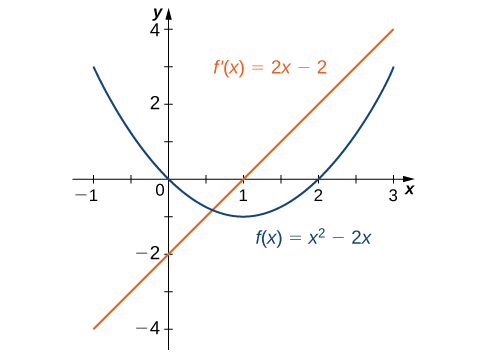
In Example \(\PageIndex{2}\), we found that for \(f(x)=x^2−2x,\; f'(x)=2x−2\). The graphs of these functions are shown in Figure \(\PageIndex{3}\). Observe that \(f(x)\) is decreasing for \(x<1\). For these same values of \(x\), \(f'(x)<0\). For values of \(x>1\), \(f(x)\) is increasing and \(f'(x)>0\). Also, \(f(x)\) has a horizontal tangent at \(x=1\) and \(f'(1)=0\).

Figure \(\PageIndex{3}\): The derivative \(f'(x)<0\) where the function \(f(x)\) is decreasing and \(f'(x)>0\) where \(f(x)\) is increasing. The derivative is zero where the function has a horizontal tangent

Example \(\PageIndex{3}\): Sketching a Derivative Using a Function

Use the following graph of \(f(x)\) to sketch a graph of \(f'(x)\).

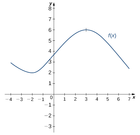
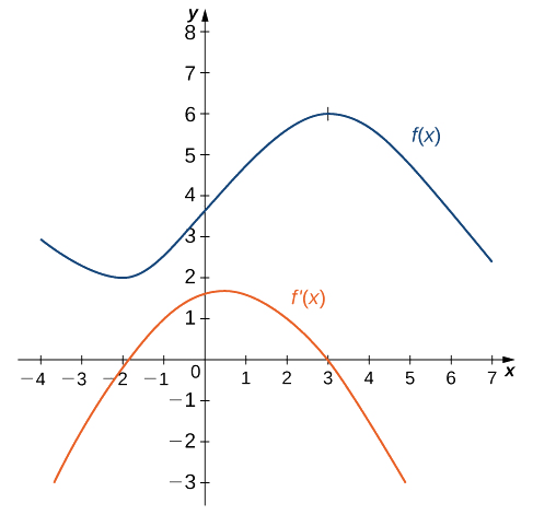
Solution

The solution is shown in the following graph. Observe that \(f(x)\) is increasing and \(f'(x)>0\) on \((–2,3)\). Also, \(f(x)\) is decreasing and \(f'(x)<0\) on \((−∞,−2)\) and on \((3,+∞)\). Also note that \(f(x)\) has horizontal tangents at \(–2\) and \(3\), and \(f'(−2)=0\) and \(f'(3)=0\).

Exercise \(\PageIndex{2}\)

Sketch the graph of \(f(x)=x^2−4\). On what interval is the graph of \(f'(x)\) above the \(x\)-axis?

Hint

The graph of \(f'(x)\) is positive where \(f(x)\) is increasing.

Answer

\((0,+∞)\)

Derivatives and Continuity

Now that we can graph a derivative, let’s examine the behavior of the graphs. First, we consider the relationship between differentiability and continuity. We will see that if a function is differentiable at a point, it must be continuous there; however, a function that is continuous at a point need not be differentiable at that point. In fact, a function may be continuous at a point and fail to be differentiable at the point for one of several reasons.

Differentiability Implies Continuity

Let \(f(x)\) be a function and \(a\) be in its domain. If \(f(x)\) is differentiable at \(a\), then \(f\) is continuous at \(a\).

Proof

If \(f(x)\) is differentiable at \(a\), then \(f'(a)\) exists and, if we let \(h = x - a\), we have \( x = a + h \), and as \(h=x-a\to 0\), we can see that \(x\to a\).

Then

\[ f'(a) = \lim_{h\to 0}\frac{f(a+h)-f(a)}{h}\nonumber\]

can be rewritten as

\(f'(a)=\displaystyle \lim_{x→a}\frac{f(x)−f(a)}{x−a}\).

We want to show that \(f(x)\) is continuous at \(a\) by showing that \(\displaystyle \lim_{x→a}f(x)=f(a).\) Thus,

\(\begin{align*} \displaystyle \lim_{x→a}f(x) &=\lim_{x→a}\;\big(f(x)−f(a)+f(a)\big)\\[4pt]
&=\lim_{x→a}\left(\frac{f(x)−f(a)}{x−a}⋅(x−a)+f(a)\right) & & \text{Multiply and divide }(f(x)−f(a))\text{ by }x−a.\\[4pt]
&=\left(\lim_{x→a}\frac{f(x)−f(a)}{x−a}\right)⋅\left( \lim_{x→a}\;(x−a)\right)+\lim_{x→a}f(a)\\[4pt]
&=f'(a)⋅0+f(a)\\[4pt]
&=f(a). \end{align*}\)

Therefore, since \(f(a)\) is defined and \(\displaystyle \lim_{x→a}f(x)=f(a)\), we conclude that \(f\) is continuous at \(a\).

□

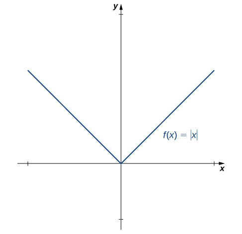
We have just proven that differentiability implies continuity, but now we consider whether continuity implies differentiability. To determine an answer to this question, we examine the function \(f(x)=|x|\). This function is continuous everywhere; however, \(f'(0)\) is undefined. This observation leads us to believe that continuity does not imply differentiability. Let’s explore further. For \(f(x)=|x|\),

\(f'(0)=\displaystyle \lim_{x→0}\frac{f(x)−f(0)}{x−0}= \lim_{x→0}\frac{|x|−|0|}{x−0}= \lim_{x→0}\frac{|x|}{x}\).

This limit does not exist because

\(\displaystyle \lim_{x→0^−}\frac{|x|}{x}=−1\) and \(\displaystyle \lim_{x→0^+}\frac{|x|}{x}=1\).

See Figure \(\PageIndex{4}\).

Figure \(\PageIndex{4}\): The function \(f(x)=|x|\) is continuous at \(0\) but is not differentiable at \(0\).

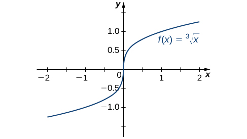
Let’s consider some additional situations in which a continuous function fails to be differentiable. Consider the function \(f(x)=\sqrt[3]{x}\):

\(f'(0)=\displaystyle \lim_{x→0}\frac{\sqrt[3]{x}−0}{x−0}=\displaystyle \lim_{x→0}\frac{1}{\sqrt[3]{x^2}}=+∞\).

Thus \(f'(0)\) does not exist. A quick look at the graph of \(f(x)=\sqrt[3]{x}\) clarifies the situation. The function has a vertical tangent line at \(0\) (Figure \(\PageIndex{5}\)).

Figure \(\PageIndex{5}\): The function \(f(x)=\sqrt[3]{x}\) has a vertical tangent at \(x=0\). It is continuous at \(0\) but is not differentiable at \(0\).

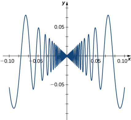
The function \(f(x)=\begin{cases} x\sin\left(\frac{1}{x}\right), & & \text{ if } x≠0\\0, & & \text{ if } x=0\end{cases}\) also has a derivative that exhibits interesting behavior at \(0\).

We see that

\(f'(0)=\displaystyle \lim_{x→0}\frac{x\sin\left(1/x\right)−0}{x−0}= \lim_{x→0}\sin\left(\frac{1}{x}\right)\).

This limit does not exist, essentially because the slopes of the secant lines continuously change direction as they approach zero (Figure \(\PageIndex{6}\)).

Figure \(\PageIndex{6}\): The function \(f(x)=\begin{cases} x\sin\left(\frac{1}{x}\right), & & \text{ if } x≠0\\0, & & \text{ if } x=0\end{cases}\) is not differentiable at \(0\).

In summary:

1. We observe that if a function is not continuous, it cannot be differentiable, since every differentiable function must be continuous. However, if a function is continuous, it may still fail to be differentiable.
2. We saw that \(f(x)=|x|\) failed to be differentiable at \(0\) because the limit of the slopes of the tangent lines on the left and right were not the same. Visually, this resulted in a sharp corner on the graph of the function at \(0.\) From this we conclude that in order to be differentiable at a point, a function must be “smooth” at that point.
3. As we saw in the example of \(f(x)=\sqrt[3]{x}\), a function fails to be differentiable at a point where there is a vertical tangent line.
4. As we saw with \(f(x)=\begin{cases}x\sin\left(\frac{1}{x}\right), & & \text{ if } x≠0\\0, & &\text{ if } x=0\end{cases}\) a function may fail to be differentiable at a point in more complicated ways as well.

Example \(\PageIndex{4}\): A Piecewise Function that is Continuous and Differentiable

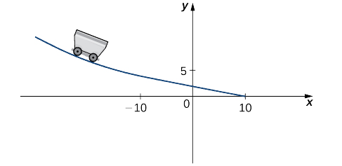
A toy company wants to design a track for a toy car that starts out along a parabolic curve and then converts to a straight line (Figure \(\PageIndex{7}\)). The function that describes the track is to have the form \(f(x)=\begin{cases}\frac{1}{10}x^2+bx+c, & & \text{ if }x<−10\\−\frac{1}{4}x+\frac{5}{2}, & & \text{ if } x≥−10\end{cases}\) where \(x\) and \(f(x)\) are in inches. For the car to move smoothly along the track, the function \(f(x)\) must be both continuous and differentiable at \(−10\). Find values of \(b\) and \(c\) that make \(f(x)\) both continuous and differentiable.

Figure \(\PageIndex{7}\): For the car to move smoothly along the track, the function must be both continuous and differentiable.

Solution

For the function to be continuous at \(x=−10\), \(\displaystyle \lim_{x→10^−}f(x)=f(−10)\). Thus, since

\(\displaystyle \lim_{x→−10^−}f(x)=\frac{1}{10}(−10)^2−10b+c=10−10b+c\)

and \(f(−10)=5\), we must have \(10−10b+c=5\). Equivalently, we have \(c=10b−5\).

For the function to be differentiable at \(−10\),

\(f'(10)=\displaystyle \lim_{x→−10}\frac{f(x)−f(−10)}{x+10}\)

must exist. Since \(f(x)\) is defined using different rules on the right and the left, we must evaluate this limit from the right and the left and then set them equal to each other:

\(\displaystyle \begin{align*} \lim_{x→−10^−}\frac{f(x)−f(−10)}{x+10} &= \lim_{x→−10^−}\frac{\frac{1}{10}x^2+bx+c−5}{x+10}\\[4pt]
&= \lim_{x→−10^−}\frac{\frac{1}{10}x^2+bx+(10b−5)−5}{x+10} & & \text{Substitute }c=10b−5.\\[4pt]
&= \lim_{x→−10^−}\frac{x^2−100+10bx+100b}{10(x+10)}\\[4pt]
&= \lim_{x→−10^−}\frac{(x+10)(x−10+10b)}{10(x+10)} & & \text{Factor by grouping}\\[4pt]
&=b−2 \end{align*}\).

We also have

\(\displaystyle \begin{align*} \lim_{x→−10^+}\frac{f(x)−f(−10)}{x+10} &= \lim_{x→−10^+}\frac{−\frac{1}{4}x+\frac{5}{2}−5}{x+10}\\[4pt]
&= \lim_{x→−10^+}\frac{−(x+10)}{4(x+10)}\\[4pt]
&=−\frac{1}{4} \end{align*}\).

This gives us \(b−2=−\frac{1}{4}\). Thus \(b=\frac{7}{4}\) and \(c=10(\frac{7}{4})−5=\frac{25}{2}\).

Exercise \(\PageIndex{3}\)

Find values of a and b that make \(f(x)=\begin{cases}ax+b, & & \text{ if } x<3\\x^2, & & \text{ if } x≥3\end{cases}\) both continuous and differentiable at \(3\).

Hint

Use Example \(\PageIndex{4}\) as a guide.

Answer

\(a=6\) and \(b=−9\)

Higher-Order Derivatives

The derivative of a function is itself a function, so we can find the derivative of a derivative. For example, the derivative of a position function is the rate of change of position, or velocity. The derivative of velocity is the rate of change of velocity, which is acceleration. The new function obtained by differentiating the derivative is called the second derivative. Furthermore, we can continue to take derivatives to obtain the third derivative, fourth derivative, and so on. Collectively, these are referred to as higher-order derivatives. The notation for the higher-order derivatives of \(y=f(x)\) can be expressed in any of the following forms:

\(f''(x),\; f'''(x),\; f^{(4)}(x),\; …\; ,\; f^{(n)}(x)\)

\(y''(x),\; y'''(x),\; y^{(4)}(x),\; …\; ,\; y^{(n)}(x)\)

\(\dfrac{d^2y}{dx^2},\;\dfrac{d^3y}{dy^3},\;\dfrac{d^4y}{dy^4},\;…\;,\;\dfrac{d^ny}{dy^n}.\)

It is interesting to note that the notation for \(\dfrac{d^2y}{dx^2}\) may be viewed as an attempt to express \(\dfrac{d}{dx}\left(\dfrac{dy}{dx}\right)\) more compactly.

Analogously, \(\dfrac{d}{dx}\left(\dfrac{d}{dx}\left(\dfrac{dy}{dx}\right)\right)=\dfrac{d}{dx}\left(\dfrac{d^2y}{dx^2}\right)=\dfrac{d^3y}{dx^3}\).

Example \(\PageIndex{5}\): Finding a Second Derivative

For \(f(x)=2x^2−3x+1\), find \(f''(x)\).

Solution

First find \(f'(x)\).

Substitute \(f(x)=2x^2−3x+1\) and \(f(x+h)=2(x+h)^2−3(x+h)+1\) into \(f'(x)=\displaystyle \lim_{h→0}\dfrac{f(x+h)−f(x)}{h}.\)

\(f'(x)=\displaystyle \lim_{h→0}\frac{(2(x+h)^2−3(x+h)+1)−(2x^2−3x+1)}{h}\)
\(=\displaystyle \lim_{h→0}\frac{4xh+h^2−3h}{h}\)	Simplify the numerator.
\(=\displaystyle \lim_{h→0}(4x+h−3)\)	Factor out the \(h\) in the numerator and cancel with the \(h\) in the denominator.
\(=4x−3\)	Take the limit.

Next, find \(f''(x)\) by taking the derivative of \(f'(x)=4x−3.\)

\(f''(x)=\displaystyle \lim_{h→0}\frac{f'(x+h)−f'(x)}{h}\)	Use \(f'(x)=\displaystyle \lim_{h→0}\frac{f(x+h)−f(x)}{h}\) with \(f ′(x)\) in place of \(f(x).\)
\(=\displaystyle \lim_{h→0}\frac{(4(x+h)−3)−(4x−3)}{h}\)	Substitute \(f'(x+h)=4(x+h)−3\) and \(f'(x)=4x−3.\)
\(=\displaystyle \lim_{h→0}4\)	Simplify.
\(=4\)	Take the limit.

Exercise \(\PageIndex{4}\)

Find \(f''(x)\) for \(f(x)=x^2\).

Hint

We found \(f'(x)=2x\) in a previous checkpoint. Use Equation \ref{derdef} to find the derivative of \(f'(x)\)

Answer

\(f''(x)=2\)

Example \(\PageIndex{6}\): Finding Acceleration

The position of a particle along a coordinate axis at time \(t\) (in seconds) is given by \(s(t)=3t^2−4t+1\) (in meters). Find the function that describes its acceleration at time \(t\).

Solution

Since \(v(t)=s′(t)\) and \(a(t)=v′(t)=s''(t)\), we begin by finding the derivative of \(s(t)\):

\(\displaystyle \begin{align*} s′(t) &= \lim_{h→0}\frac{s(t+h)−s(t)}{h}\\[4pt]
&=\lim_{h→0}\frac{3(t+h)^2−4(t+h)+1−(3t^2−4t+1)}{h}\\[4pt]
&=6t−4. \end{align*}\)

Next,

\(\displaystyle \begin{align*} s''(t)&= \lim_{h→0}\frac{s′(t+h)−s′(t)}{h}\\[4pt]
&=\lim_{h→0}\frac{6(t+h)−4−(6t−4)}{h}\\[4pt]
&=6. \end{align*}\)

Thus, \(a=6 \;\text{m/s}^2\).

Exercise \(\PageIndex{5}\)

For \(s(t)=t^3\), find \(a(t).\)

Hint

Use Example \(\PageIndex{6}\) as a guide.

Answer

\(a(t)=6t\)

 

Key Concepts

• The slope of the tangent line to a curve measures the instantaneous rate of change of a curve. We can calculate it by finding the limit of the difference quotient or the difference quotient with increment \(h\).
• The derivative of a function \(f(x)\) at a value \(a\) is found using either of the definitions for the slope of the tangent line.
• Velocity is the rate of change of position. As such, the velocity \(v(t)\) at time \(t\) is the derivative of the position \(s(t)\) at time \(t\).
  Average velocity is given by \[v_{ave}=\dfrac{s(t)−s(a)}{t−a}. \nonumber\] Instantaneous velocity is given by \[\displaystyle v(a)=s′(a)=\lim_{t→a}\frac{s(t)−s(a)}{t−a}. \nonumber\]
• We may estimate a derivative by using a table of values.
• The derivative of a function \(f(x)\) is the function whose value at \(x\) is \(f'(x)\).
• The graph of a derivative of a function \(f(x)\) is related to the graph of \(f(x)\). Where \(f(x)\) has a tangent line with positive slope, \(f'(x)>0\). Where \(f(x)\) has a tangent line with negative slope, \(f'(x)<0\). Where \(f(x)\) has a horizontal tangent line, \(f'(x)=0.\)
• If a function is differentiable at a point, then it is continuous at that point. A function is not differentiable at a point if it is not continuous at the point, if it has a vertical tangent line at the point, or if the graph has a sharp corner or cusp.
• Higher-order derivatives are derivatives of derivatives, from the second derivative to the \(n^{\text{th}}\) derivative.

Key Equations

• Difference quotient

\(Q=\dfrac{f(x)−f(a)}{x−a}\)

• Difference quotient with increment h

\(Q=\dfrac{f(a+h)−f(a)}{a+h−a}=\dfrac{f(a+h)−f(a)}{h}\)

• Slope of tangent line

\(\displaystyle m_{tan}=\lim_{x→a}\frac{f(x)−f(a)}{x−a}\)

\(\displaystyle m_{tan}=\lim_{h→0}\frac{f(a+h)−f(a)}{h}\)

• Derivative of f(x) at a

\(\displaystyle f′(a)=\lim_{x→a}\frac{f(x)−f(a)}{x−a}\)

\(\displaystyle f′(a)=\lim_{h→0}\frac{f(a+h)−f(a)}{h}\)

• Average velocity

\(v_{ave}=\dfrac{s(t)−s(a)}{t−a}\)

• Instantaneous velocity

\(\displaystyle v(a)=s′(a)=\lim_{t→a}\frac{s(t)−s(a)}{t−a}\)

• The derivative function

\(f'(x)=\displaystyle \lim_{h→0}\frac{f(x+h)−f(x)}{h}\)

Glossary

derivative

the slope of the tangent line to a function at a point, calculated by taking the limit of the difference quotient, is the derivative

difference quotient

of a function \(f(x)\) at \(a\) is given by

\(\dfrac{f(a+h)−f(a)}{h}\) or \(\dfrac{f(x)−f(a)}{x−a}\)

differentiation

the process of taking a derivative

instantaneous rate of change

the rate of change of a function at any point along the function \(a\), also called \(f′(a)\), or the derivative of the function at \(a\)

derivative function

gives the derivative of a function at each point in the domain of the original function for which the derivative is defined

differentiable at \(a\)

a function for which \(f'(a)\) exists is differentiable at \(a\)

differentiable on \(S\)

a function for which \(f'(x)\) exists for each \(x\) in the open set \(S\) is differentiable on \(S\)

differentiable function

a function for which \(f'(x)\) exists is a differentiable function

higher-order derivative

a derivative of a derivative, from the second derivative to the \(n^{\text{th}}\) derivative, is called a higher-order derivative

Contributors and Attributions

• Gilbert Strang (MIT) and Edwin “Jed” Herman (Harvey Mudd) with many contributing authors. This content by OpenStax is licensed with a CC-BY-SA-NC 4.0 license. Download for free at http://cnx.org.

• Gilbert Strang (MIT) and Edwin “Jed” Herman (Harvey Mudd) with many contributing authors. This content by OpenStax is licensed with a CC-BY-SA-NC 4.0 license. Download for free at http://cnx.org.

• Paul Seeburger (Monroe Community College) added explanation of the alternative definition of the derivative used in the proof of that differentiability implies continuity.