
11.8: Vectors
- Page ID
- 119209

\( \newcommand{\vecs}[1]{\overset { \scriptstyle \rightharpoonup} {\mathbf{#1}} } \)
\( \newcommand{\vecd}[1]{\overset{-\!-\!\rightharpoonup}{\vphantom{a}\smash {#1}}} \)
\( \newcommand{\dsum}{\displaystyle\sum\limits} \)
\( \newcommand{\dint}{\displaystyle\int\limits} \)
\( \newcommand{\dlim}{\displaystyle\lim\limits} \)
\( \newcommand{\id}{\mathrm{id}}\) \( \newcommand{\Span}{\mathrm{span}}\)
( \newcommand{\kernel}{\mathrm{null}\,}\) \( \newcommand{\range}{\mathrm{range}\,}\)
\( \newcommand{\RealPart}{\mathrm{Re}}\) \( \newcommand{\ImaginaryPart}{\mathrm{Im}}\)
\( \newcommand{\Argument}{\mathrm{Arg}}\) \( \newcommand{\norm}[1]{\| #1 \|}\)
\( \newcommand{\inner}[2]{\langle #1, #2 \rangle}\)
\( \newcommand{\Span}{\mathrm{span}}\)
\( \newcommand{\id}{\mathrm{id}}\)
\( \newcommand{\Span}{\mathrm{span}}\)
\( \newcommand{\kernel}{\mathrm{null}\,}\)
\( \newcommand{\range}{\mathrm{range}\,}\)
\( \newcommand{\RealPart}{\mathrm{Re}}\)
\( \newcommand{\ImaginaryPart}{\mathrm{Im}}\)
\( \newcommand{\Argument}{\mathrm{Arg}}\)
\( \newcommand{\norm}[1]{\| #1 \|}\)
\( \newcommand{\inner}[2]{\langle #1, #2 \rangle}\)
\( \newcommand{\Span}{\mathrm{span}}\) \( \newcommand{\AA}{\unicode[.8,0]{x212B}}\)
\( \newcommand{\vectorA}[1]{\vec{#1}} % arrow\)
\( \newcommand{\vectorAt}[1]{\vec{\text{#1}}} % arrow\)
\( \newcommand{\vectorB}[1]{\overset { \scriptstyle \rightharpoonup} {\mathbf{#1}} } \)
\( \newcommand{\vectorC}[1]{\textbf{#1}} \)
\( \newcommand{\vectorD}[1]{\overrightarrow{#1}} \)
\( \newcommand{\vectorDt}[1]{\overrightarrow{\text{#1}}} \)
\( \newcommand{\vectE}[1]{\overset{-\!-\!\rightharpoonup}{\vphantom{a}\smash{\mathbf {#1}}}} \)
\( \newcommand{\vecs}[1]{\overset { \scriptstyle \rightharpoonup} {\mathbf{#1}} } \)
\(\newcommand{\longvect}{\overrightarrow}\)
\( \newcommand{\vecd}[1]{\overset{-\!-\!\rightharpoonup}{\vphantom{a}\smash {#1}}} \)
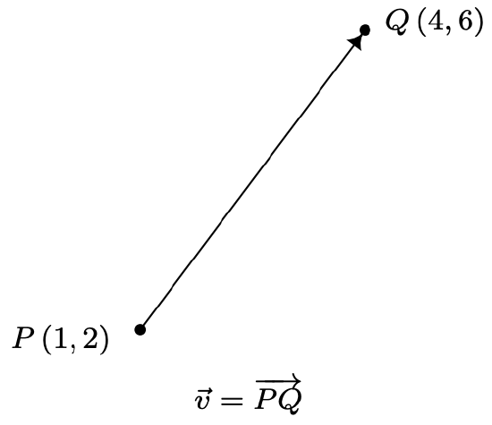
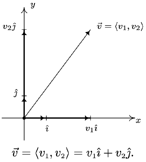
\(\newcommand{\avec}{\mathbf a}\) \(\newcommand{\bvec}{\mathbf b}\) \(\newcommand{\cvec}{\mathbf c}\) \(\newcommand{\dvec}{\mathbf d}\) \(\newcommand{\dtil}{\widetilde{\mathbf d}}\) \(\newcommand{\evec}{\mathbf e}\) \(\newcommand{\fvec}{\mathbf f}\) \(\newcommand{\nvec}{\mathbf n}\) \(\newcommand{\pvec}{\mathbf p}\) \(\newcommand{\qvec}{\mathbf q}\) \(\newcommand{\svec}{\mathbf s}\) \(\newcommand{\tvec}{\mathbf t}\) \(\newcommand{\uvec}{\mathbf u}\) \(\newcommand{\vvec}{\mathbf v}\) \(\newcommand{\wvec}{\mathbf w}\) \(\newcommand{\xvec}{\mathbf x}\) \(\newcommand{\yvec}{\mathbf y}\) \(\newcommand{\zvec}{\mathbf z}\) \(\newcommand{\rvec}{\mathbf r}\) \(\newcommand{\mvec}{\mathbf m}\) \(\newcommand{\zerovec}{\mathbf 0}\) \(\newcommand{\onevec}{\mathbf 1}\) \(\newcommand{\real}{\mathbb R}\) \(\newcommand{\twovec}[2]{\left[\begin{array}{r}#1 \\ #2 \end{array}\right]}\) \(\newcommand{\ctwovec}[2]{\left[\begin{array}{c}#1 \\ #2 \end{array}\right]}\) \(\newcommand{\threevec}[3]{\left[\begin{array}{r}#1 \\ #2 \\ #3 \end{array}\right]}\) \(\newcommand{\cthreevec}[3]{\left[\begin{array}{c}#1 \\ #2 \\ #3 \end{array}\right]}\) \(\newcommand{\fourvec}[4]{\left[\begin{array}{r}#1 \\ #2 \\ #3 \\ #4 \end{array}\right]}\) \(\newcommand{\cfourvec}[4]{\left[\begin{array}{c}#1 \\ #2 \\ #3 \\ #4 \end{array}\right]}\) \(\newcommand{\fivevec}[5]{\left[\begin{array}{r}#1 \\ #2 \\ #3 \\ #4 \\ #5 \\ \end{array}\right]}\) \(\newcommand{\cfivevec}[5]{\left[\begin{array}{c}#1 \\ #2 \\ #3 \\ #4 \\ #5 \\ \end{array}\right]}\) \(\newcommand{\mattwo}[4]{\left[\begin{array}{rr}#1 \amp #2 \\ #3 \amp #4 \\ \end{array}\right]}\) \(\newcommand{\laspan}[1]{\text{Span}\{#1\}}\) \(\newcommand{\bcal}{\cal B}\) \(\newcommand{\ccal}{\cal C}\) \(\newcommand{\scal}{\cal S}\) \(\newcommand{\wcal}{\cal W}\) \(\newcommand{\ecal}{\cal E}\) \(\newcommand{\coords}[2]{\left\{#1\right\}_{#2}}\) \(\newcommand{\gray}[1]{\color{gray}{#1}}\) \(\newcommand{\lgray}[1]{\color{lightgray}{#1}}\) \(\newcommand{\rank}{\operatorname{rank}}\) \(\newcommand{\row}{\text{Row}}\) \(\newcommand{\col}{\text{Col}}\) \(\renewcommand{\row}{\text{Row}}\) \(\newcommand{\nul}{\text{Nul}}\) \(\newcommand{\var}{\text{Var}}\) \(\newcommand{\corr}{\text{corr}}\) \(\newcommand{\len}[1]{\left|#1\right|}\) \(\newcommand{\bbar}{\overline{\bvec}}\) \(\newcommand{\bhat}{\widehat{\bvec}}\) \(\newcommand{\bperp}{\bvec^\perp}\) \(\newcommand{\xhat}{\widehat{\xvec}}\) \(\newcommand{\vhat}{\widehat{\vvec}}\) \(\newcommand{\uhat}{\widehat{\uvec}}\) \(\newcommand{\what}{\widehat{\wvec}}\) \(\newcommand{\Sighat}{\widehat{\Sigma}}\) \(\newcommand{\lt}{<}\) \(\newcommand{\gt}{>}\) \(\newcommand{\amp}{&}\) \(\definecolor{fillinmathshade}{gray}{0.9}\)As we have seen numerous times in this book, Mathematics can be used to model and solve real-world problems. For many applications, real numbers suffice; that is, real numbers with the appropriate units attached can be used to answer questions like “How close is the nearest Sasquatch nest?” There are other times though, when these kinds of quantities do not suffice. Perhaps it is important to know, for instance, how close the nearest Sasquatch nest is as well as the direction in which it lies. (Foreshadowing the use of bearings in the exercises, perhaps?) To answer questions like these which involve both a quantitative answer, or magnitude, along with a direction, we use the mathematical objects called vectors.1 A vector is represented geometrically as a directed line segment where the magnitude of the vector is taken to be the length of the line segment and the direction is made clear with the use of an arrow at one endpoint of the segment. When referring to vectors in this text, we shall adopt2 the ‘arrow’ notation, so the symbol \(\vec{v}\) is read as ‘the vector \(v^{\prime}\). Below is a typical vector \(\vec{v}\) with endpoints \(P\) (1, 2) and \(Q\) (4, 6). The point \(P\) is called the initial point or tail of \(\vec{v}\) and the point \(Q\) is called the terminal point or head of \(\vec{v}\). Since we can reconstruct \(\vec{v}\) completely from \(P\) and \(Q\), we write \(\vec{v}=\overrightarrow{P Q}\), where the order of points \(P\) (initial point) and \(Q\) (terminal point) is important. (Think about this before moving on.)
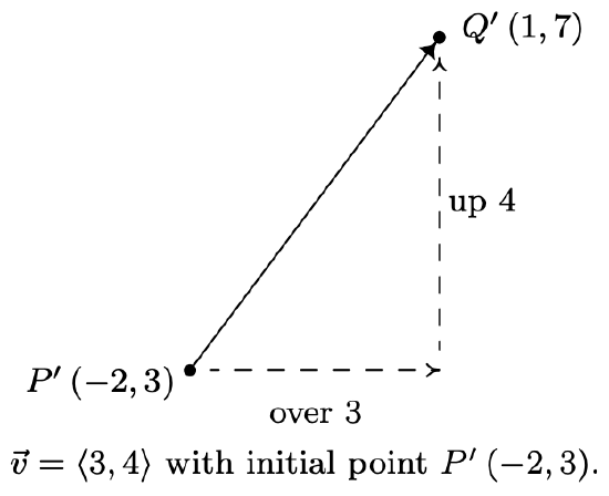
While it is true that \(P\) and \(Q\) completely determine \(\vec{v}\), it is important to note that since vectors are defined in terms of their two characteristics, magnitude and direction, any directed line segment with the same length and direction as \(\vec{v}\) is considered to be the same vector as \(\vec{v}\), regardless of its initial point. In the case of our vector \(\vec{v}\) above, any vector which moves three units to the right and four up3 from its initial point to arrive at its terminal point is considered the same vector as \(\vec{v}\). The notation we use to capture this idea is the component form of the vector, \(\vec{v}=\langle 3,4\rangle\), where the first number, 3, is called the \(x\)-component of \(\vec{v}\) and the second number, 4, is called the \(y\)-component of \(\vec{v}\). If we wanted to reconstruct \(\vec{v}=\langle 3,4\rangle\) with initial point \(P^{\prime}(-2,3)\), then we would find the terminal point of \(\vec{v}\) by adding 3 to the \(x\)-coordinate and adding 4 to the \(y\)-coordinate to obtain the terminal point \(Q^{\prime}(1,7)\), as seen below.
The component form of a vector is what ties these very geometric objects back to Algebra and ultimately Trigonometry. We generalize our example in our definition below.
Suppose \(\vec{v}\) is represented by a directed line segment with initial point \(P\left(x_{0}, y_{0}\right)\) and terminal point \(Q\left(x_{1}, y_{1}\right)\). The component form of \(\vec{v}\) is given by
\[\vec{v}=\overrightarrow{P Q}=\left\langle x_{1}-x_{0}, y_{1}-y_{0}\right\rangle\nonumber\]
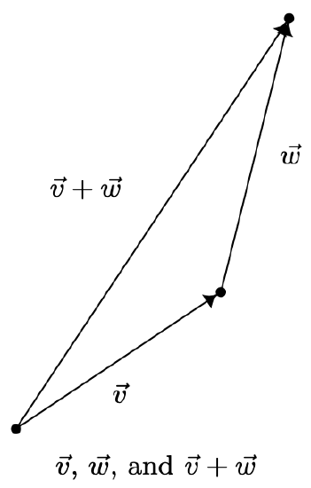
Using the language of components, we have that two vectors are equal if and only if their corresponding components are equal. That is, \(\left\langle v_{1}, v_{2}\right\rangle=\left\langle v_{1}^{\prime}, v_{2}^{\prime}\right\rangle\) if and only if \(v_{1}=v_{1}^{\prime}\) and \(v_{2}=v_{2}^{\prime}\). (Again, think about this before reading on.) We now set about defining operations on vectors. Suppose we are given two vectors \(\vec{v}\) and \(\vec{w}\). The sum, or resultant vector \(\vec{v}+\vec{w}\) is obtained as follows. First, plot \(\vec{v}\). Next, plot \(\vec{w}\) so that its initial point is the terminal point of \(\vec{v}\). To plot the vector \(\vec{v}+\vec{w}\) we begin at the initial point of \(\vec{v}\) and end at the terminal point of \(\vec{w}\). It is helpful to think of the vector \(\vec{v}+\vec{w}\) as the ‘net result’ of moving along \(\vec{v}\) then moving along \(\vec{w}\).
Our next example makes good use of resultant vectors and reviews bearings and the Law of Cosines.4
A plane leaves an airport with an airspeed5 of 175 miles per hour at a bearing of \(\mathrm{N} 40^{\circ} \mathrm{E}\). A 35 mile per hour wind is blowing at a bearing of \(\mathrm{S} 60^{\circ} \mathrm{E}\). Find the true speed of the plane, rounded to the nearest mile per hour, and the true bearing of the plane, rounded to the nearest degree.
Solution
For both the plane and the wind, we are given their speeds and their directions. Coupling speed (as a magnitude) with direction is the concept of velocity which we’ve seen a few times before in this textbook.6 We let \(\vec{v}\) denote the plane’s velocity and \(\vec{w}\) denote the wind’s velocity in the diagram below. The ‘true’ speed and bearing is found by analyzing the resultant vector, \(\vec{v}+\vec{w}\). From the vector diagram, we get a triangle, the lengths of whose sides are the magnitude of \(\vec{v}\), which is 175, the magnitude of \(\vec{w}\), which is 35, and the magnitude of \(\vec{v}+\vec{w}\), which we’ll call \(c\). From the given bearing information, we go through the usual geometry to determine that the angle between the sides of length 35 and 175 measures \(100^{\circ}\).

From the Law of Cosines, we determine \(c=\sqrt{31850-12250 \cos \left(100^{\circ}\right)} \approx 184\), which means the true speed of the plane is (approximately) 184 miles per hour. To determine the true bearing of the plane, we need to determine the angle \(\alpha\). Using the Law of Cosines once more,7 we find \(\cos (\alpha)=\frac{c^{2}+29400}{350 c}\) so that \(\alpha \approx 11^{\circ}\). Given the geometry of the situation, we add \(\alpha\) to the given \(40^{\circ}\) and find the true bearing of the plane to be (approximately) \(\mathrm{N} 51^{\circ} \mathrm{E}\).
Our next step is to define addition of vectors component-wise to match the geometric action.8
Suppose \(\vec{v}=\left\langle v_{1}, v_{2}\right\rangle\) and \(\vec{w}=\left\langle w_{1}, w_{2}\right\rangle\). The vector \(\vec{v}+\vec{w}\) is defined by
\(\vec{v}+\vec{w}=\left\langle v_{1}+w_{1}, v_{2}+w_{2}\right\rangle\)
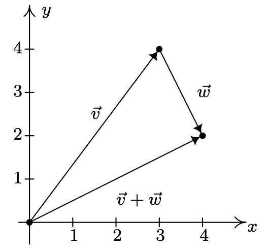
Let \(\vec{v}=\langle 3,4\rangle\) and suppose \(\vec{w}=\overrightarrow{P Q}\) where \(P(−3, 7)\) and \(Q(−2, 5)\). Find \(\vec{v}+\vec{w}\) and interpret this sum geometrically.
Solution
Before can add the vectors using Definition 11.6, we need to write \(\vec{w}\) in component form. Using Definition 11.5, we get \(\vec{w}=\langle-2-(-3), 5-7\rangle=\langle 1,-2\rangle\). Thus
\[\begin{aligned}
\vec{v}+\vec{w} &=\langle 3,4\rangle+\langle 1,-2\rangle \\
&=\langle 3+1,4+(-2)\rangle \\
&=\langle 4,2\rangle
\end{aligned}\nonumber\]
To visualize this sum, we draw \(\vec{v}\) with its initial point at (0, 0) (for convenience) so that its terminal point is (3, 4). Next, we graph \(\vec{w}\) with its initial point at (3, 4). Moving one to the right and two down, we find the terminal point of \(\vec{w}\) to be (4, 2). We see that the vector \(\vec{v}+\vec{w}\) has initial point (0, 0) and terminal point (4, 2) so its component form is \(\langle 4,2\rangle\), as required.
In order for vector addition to enjoy the same kinds of properties as real number addition, it is necessary to extend our definition of vectors to include a ‘zero vector’, \(\overrightarrow{0}=\langle 0,0\rangle\). Geometrically, \(\overrightarrow{0}\) represents a point, which we can think of as a directed line segment with the same initial and terminal points. The reader may well object to the inclusion of \(\overrightarrow{0}\), since after all, vectors are supposed to have both a magnitude (length) and a direction. While it seems clear that the magnitude of \(\overrightarrow{0}\) should be 0, it is not clear what its direction is. As we shall see, the direction of \(\overrightarrow{0}\) is in fact undefined, but this minor hiccup in the natural flow of things is worth the benefits we reap by including \(\overrightarrow{0}\) in our discussions. We have the following theorem.
- Commutative Property: For all vectors \(\vec{v}\) and \(\vec{w}, \vec{v}+\vec{w}=\vec{w}+\vec{v}\).
- Associative Property: For all vectors \(\vec{u}, \vec{v} \text { and } \vec{w},(\vec{u}+\vec{v})+\vec{w}=\vec{u}+(\vec{v}+\vec{w})\).
- Identity Property: The vector \(\overrightarrow{0}\) acts as the additive identity for vector addition. That is, for all vectors \(\vec{v}\), \[\vec{v}+\overrightarrow{0}=\overrightarrow{0}+\vec{v}=\vec{v}.\nonumber\]
- Inverse Property: Every vector \(\vec{v}\) has a unique additive inverse, denoted \(-\vec{v}\). That is, for every vector \(\vec{v}\), there is a vector \(-\vec{v}\) so that \[\vec{v}+(-\vec{v})=(-\vec{v})+\vec{v}=\overrightarrow{0}\nonumber\]
The properties in Theorem 11.18 are easily verified using the definition of vector addition.9 For the commutative property, we note that if \(\vec{v}=\left\langle v_{1}, v_{2}\right\rangle\) and \(\vec{w}=\left\langle w_{1}, w_{2}\right\rangle\) then
\(\begin{aligned} \vec{v}+\vec{w} &=\left\langle v_{1}, v_{2}\right\rangle+\left\langle w_{1}, w_{2}\right\rangle \\ &=\left\langle v_{1}+w_{1}, v_{2}+w_{2}\right\rangle \\ &=\left\langle w_{1}+v_{1}, w_{2}+v_{2}\right\rangle \\ &=\vec{w}+\vec{v} \end{aligned}\)
Geometrically, we can ‘see’ the commutative property by realizing that the sums \(\vec{v}+\vec{w}\) and \(\vec{w}+\vec{v}\) are the same directed diagonal determined by the parallelogram below.
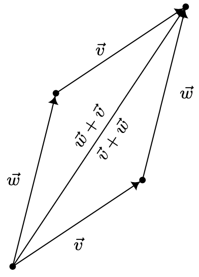 Demonstrating the commutative property of vector addition.
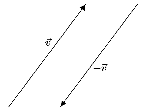
The proofs of the associative and identity properties proceed similarly, and the reader is encouraged to verify them and provide accompanying diagrams. The existence and uniqueness of the additive inverse is yet another property inherited from the real numbers. Given a vector \(\vec{v}=\left\langle v_{1}, v_{2}\right\rangle\), suppose we wish to find a vector \(\vec{w}=\left\langle w_{1}, w_{2}\right\rangle\) so that \(\vec{v}+\vec{w}=\overrightarrow{0}\). By the definition of vector addition, we have \(\left\langle v_{1}+w_{1}, v_{2}+w_{2}\right\rangle=\langle 0,0\rangle\), and hence, \(v_{1}+w_{1}=0\) and \(v_{2}+w_{2}=0\). We get \(w_{1}=-v_{1}\) and \(w_{2}=-v_{2}\) so that \(\vec{w}=\left\langle-v_{1},-v_{2}\right\rangle\). Hence, \(\vec{v}\) has an additive inverse, and moreover, it is unique and can be obtained by the formula \(-\vec{v}=\left\langle-v_{1},-v_{2}\right\rangle\). Geometrically, the vectors \(\vec{v}=\left\langle v_{1}, v_{2}\right\rangle\) and \(-\vec{v}=\left\langle-v_{1},-v_{2}\right\rangle\) have the same length, but opposite directions. As a result, when adding the vectors geometrically, the sum \(\vec{v}+(-\vec{v})\) results in starting at the initial point of \(\vec{v}\) and ending back at the initial point of \(\vec{v}\), or in other words, the net result of moving \(\vec{v}\) then \(-\vec{v}\) is not moving at all.
Using the additive inverse of a vector, we can define the difference of two vectors, \(\vec{v}-\vec{w}=\vec{v}+(-\vec{w})\). If \(\vec{v}=\left\langle v_{1}, v_{2}\right\rangle\) and \(\vec{w}=\left\langle w_{1}, w_{2}\right\rangle\) then
\(\begin{aligned} \vec{v}-\vec{w} &=\vec{v}+(-\vec{w}) \\ &=\left\langle v_{1}, v_{2}\right\rangle+\left\langle-w_{1},-w_{2}\right\rangle \\ &=\left\langle v_{1}+\left(-w_{1}\right), v_{2}+\left(-w_{2}\right)\right\rangle \\ &=\left\langle v_{1}-w_{1}, v_{2}-w_{2}\right\rangle \end{aligned}\)
In other words, like vector addition, vector subtraction works component-wise. To interpret the vector \(\vec{v}-\vec{w}\) geometrically, we note
\(\begin{array}{l} \vec{w}+(\vec{v}-\vec{w}) &=\vec{w}+(\vec{v}+(-\vec{w})) & \text { Definition of Vector Subtraction } \\ &=\vec{w}+((-\vec{w})+\vec{v}) & \text { Commutativity of Vector Addition } \\ &=(\vec{w}+(-\vec{w}))+\vec{v} & \text { Associativity of Vector Addition } \\ &=\overrightarrow{0}+\vec{v} & \text { Definition of Additive Inverse } \\ &=\vec{v} & \text { Definition of Additive Identity } \end{array}\)
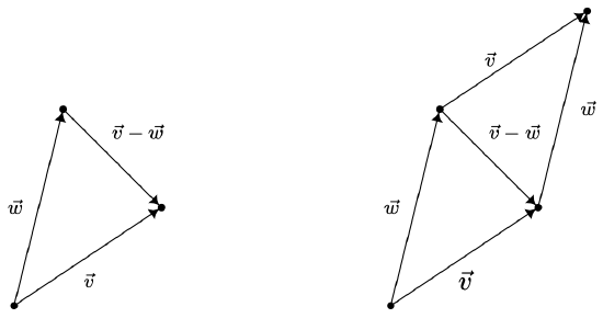
This means that the ‘net result’ of moving along \(\vec{w}\) then moving along \(\vec{v}-\vec{w}\) is just \(\vec{v}\) itself. From the diagram below, we see that \(\vec{v}-\vec{w}\) may be interpreted as the vector whose initial point is the terminal point of \(\vec{w}\) and whose terminal point is the terminal point of \(\vec{v}\) as depicted below. It is also worth mentioning that in the parallelogram determined by the vectors \(\vec{v}\) and \(\vec{w}\), the vector \(\vec{v}-\vec{w}\) is one of the diagonals – the other being \(\vec{v}+\vec{w}\).
Next, we discuss scalar multiplication – that is, taking a real number times a vector. We define scalar multiplication for vectors in the same way we defined it for matrices in Section 8.3.
If \(k\) is a real number and \(\vec{v}=\left\langle v_{1}, v_{2}\right\rangle\), we define \(k \vec{v}\) by \[k \vec{v}=k\left\langle v_{1}, v_{2}\right\rangle=\left\langle k v_{1}, k v_{2}\right\rangle\nonumber\]
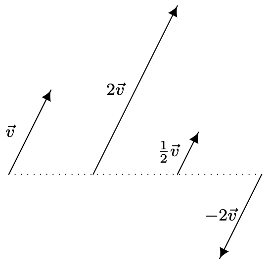
Scalar multiplication by \(k\) in vectors can be understood geometrically as scaling the vector (if \(k > 0\)) or scaling the vector and reversing its direction (if \(k < 0\)) as demonstrated below.
Note that, by definition 11.7, \((-1) \vec{v}=(-1)\left\langle v_{1}, v_{2}\right\rangle=\left\langle(-1) v_{1},(-1) v_{2}\right\rangle=\left\langle-v_{1},-v_{2}\right\rangle=-\vec{v}\). This, and other properties of scalar multiplication are summarized below.
- Associative Property: For every vector \(\vec{v}\) and scalars \(k\) and \(r\), \((k r) \vec{v}=k(r \vec{v})\).
- Identity Property: For all vectors \(\vec{v}, 1 \vec{v}=\vec{v}\).
- Additive Inverse Property: For all vectors \(\vec{v},-\vec{v}=(-1) \vec{v}\).
- Distributive Property of Scalar Multiplication over Scalar Addition: For every vector \(\vec{v}\) and scalars \(k\) and \(r\), \[(k+r) \vec{v}=k \vec{v}+r \vec{v}\nonumber\]
- Distributive Property of Scalar Multiplication over Vector Addition: For all vectors \(\vec{v}\) and \(\vec{w}\) and scalars \(k\), \[k(\vec{v}+\vec{w})=k \vec{v}+k \vec{w}\nonumber\]
- Zero Product Property: If \(\vec{v}\) is vector and \(k\) is a scalar, then \[k \vec{v}=\overrightarrow{0} \quad \text { if and only if } \quad k=0 \quad \text { or } \quad \vec{v}=\overrightarrow{0}\nonumber\]
The proof of Theorem 11.19, like the proof of Theorem 11.18, ultimately boils down to the definition of scalar multiplication and properties of real numbers. For example, to prove the associative property, we let \(\vec{v}=\left\langle v_{1}, v_{2}\right\rangle\). If \(k\) and \(r\) are scalars then
\(\begin{aligned} (k r) \vec{v} &=(k r)\left\langle v_{1}, v_{2}\right\rangle & & \\ &=\left\langle(k r) v_{1},(k r) v_{2}\right\rangle & & \text { Definition of Scalar Multiplication } \\ &=\left\langle k\left(r v_{1}\right), k\left(r v_{2}\right)\right\rangle & & \text { Associative Property of Real Number Multiplication } \\ &=k\left\langle r v_{1}, r v_{2}\right\rangle & & \text { Definition of Scalar Multiplication } \\ &=k\left(r\left\langle v_{1}, v_{2}\right\rangle\right) & & \text { Definition of Scalar Multiplication } \\ &=k(r \vec{v}) & & \end{aligned}\)
The remaining properties are proved similarly and are left as exercises.
Our next example demonstrates how Theorem 11.19 allows us to do the same kind of algebraic manipulations with vectors as we do with variables – multiplication and division of vectors notwithstanding. If the pedantry seems familiar, it should. This is the same treatment we gave Example 8.3.1 in Section 8.3. As in that example, we spell out the solution in excruciating detail to encourage the reader to think carefully about why each step is justified.
Solve \(5 \vec{v}-2(\vec{v}+\langle 1,-2\rangle)=\overrightarrow{0} \text { for } \vec{v}\).
Solution
\(\begin{aligned}
5 \vec{v}-2(\vec{v}+\langle 1,-2\rangle) &=\overrightarrow{0} \\
5 \vec{v}+(-1)[2(\vec{v}+\langle 1,-2\rangle)] &=\overrightarrow{0} \\
5 \vec{v}+[(-1)(2)](\vec{v}+\langle 1,-2\rangle) &=\overrightarrow{0} \\
5 \vec{v}+(-2)(\vec{v}+\langle 1,-2\rangle) &=\overrightarrow{0} \\
5 \vec{v}+[(-2) \vec{v}+(-2)\langle 1,-2\rangle] &=\overrightarrow{0} \\
5 \vec{v}+[(-2) \vec{v}+\langle(-2)(1),(-2)(-2)\rangle] &=\overrightarrow{0} \\
{[5 \vec{v}+(-2) \vec{v}]+\langle-2,4\rangle } &=\overrightarrow{0} \\
(5+(-2)) \vec{v}+\langle-2,4\rangle &=\overrightarrow{0} \\
3 \vec{v}+\langle-2,4\rangle &=\overrightarrow{0} \\
(3 \vec{v}+\langle-2,4\rangle)+(-\langle-2,4\rangle) &=\overrightarrow{0}+(-\langle-2,4\rangle) \\
3 \vec{v}+[\langle-2,4\rangle+(-\langle-2,4\rangle)] &=\overrightarrow{0}+(-1)\langle-2,4\rangle \\
3 \vec{v}+\overrightarrow{0} &=\overrightarrow{0}+\langle(-1)(-2),(-1)(4)\rangle \\
3 \vec{v} &=\langle 2,-4\rangle \\
\frac{1}{3}(3 \vec{v}) &=\frac{1}{3}(\langle 2,-4\rangle) \\
{\left[\left(\frac{1}{3}\right)(3)\right] \vec{v} } &=\left\langle\left(\frac{1}{3}\right)(2),\left(\frac{1}{3}\right)(-4)\right\rangle \\
1 \vec{v} &=\left\langle\frac{2}{3},-\frac{4}{3}\right\rangle \\
\vec{v} &=\left\langle\frac{2}{3},-\frac{4}{3}\right\rangle
\end{aligned}\)
A vector whose initial point is (0, 0) is said to be in standard position. If \(\vec{v}=\left\langle v_{1}, v_{2}\right\rangle\) is plotted in standard position, then its terminal point is necessarary \(\left(v_{1}, v_{2}\right)\). (Once more, think about this before reading on.)
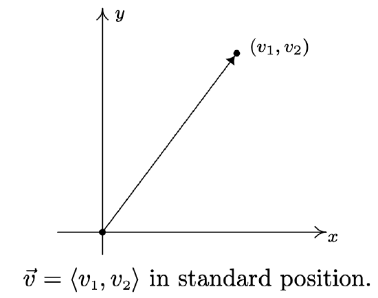
Plotting a vector in standard position enables us to more easily quantify the concepts of magnitude and direction of the vector. We can convert the point \(\left(v_{1}, v_{2}\right)\) in rectangular coordinates to a pair \((r, \theta)\) in polar coordinates where \(r \geq 0\). The magnitude of \(\vec{v}\), which we said earlier was length of the directed line segment, is \(r=\sqrt{v_{1}^{2}+v_{2}^{2}}\) and is denoted by \(\|\vec{v}\|\). From Section 11.4, we know \(v_{1}=r \cos (\theta)=\|\vec{v}\| \cos (\theta)\) and \(v_{2}=r \sin (\theta)=\|\vec{v}\| \sin (\theta)\). From the definition of scalar multiplication and vector equality, we get
\(\begin{aligned} \vec{v} &=\left\langle v_{1}, v_{2}\right\rangle \\ &=\langle\|\vec{v}\| \cos (\theta),\|\vec{v}\| \sin (\theta)\rangle \\ &=\|\vec{v}\|\langle\cos (\theta), \sin (\theta)\rangle \end{aligned}\)
This motivates the following definition.
Suppose \(\vec{v}\) is a vector with component form \(\vec{v}=\left\langle v_{1}, v_{2}\right\rangle\). Let \((r, \theta)\) be a polar representation of the point with rectangular coordinates \(\left(v_{1}, v_{2}\right)\) with \(r \geq 0\).
- The magnitude of \(\vec{v}\), denoted \(\|\vec{v}\|\), is given by \(\|\vec{v}\|=r=\sqrt{v_{1}^{2}+v_{2}^{2}}\)
- If \(\vec{v} \neq \overrightarrow{0}\), the (vector) direction of \(\vec{v}\), denoted \(\hat{v}\) is given by \(\hat{v}=\langle\cos (\theta), \sin (\theta)\rangle\)
Taken together, we get \(\vec{v}=\langle\|\vec{v}\| \cos (\theta),\|\vec{v}\| \sin (\theta)\rangle\).
A few remarks are in order. First, we note that if \(\vec{v} \neq 0\) then even though there are infinitely many angles \(\theta\) which satisfy Definition 11.8, the stipulation \(r > 0\) means that all of the angles are coterminal. Hence, if \(\theta\) and \(\theta^{\prime}\) both satisfy the conditions of Definition 11.8, then \(\cos (\theta)=\cos \left(\theta^{\prime}\right)\) and \(\sin (\theta)=\sin \left(\theta^{\prime}\right)\), and as such, \(\langle\cos (\theta), \sin (\theta)\rangle=\left\langle\cos \left(\theta^{\prime}\right), \sin \left(\theta^{\prime}\right)\right\rangle\) making \(\hat{v}\) is well-defined.10 If \(\vec{v}=\overrightarrow{0}\), then \(\vec{v}=\langle 0,0\rangle\), and we know from Section 11.4 that \((0, \theta)\) is a polar representation for the origin for any angle \(\theta\). For this reason, \(\hat{0}\) is undefined. The following theorem summarizes the important facts about the magnitude and direction of a vector.
Suppose \(\vec{v}\) is a vector.
- \(\|\vec{v}\| \geq 0\) and \(\|\vec{v}\|=0\) if and only if \(\vec{v}=\overrightarrow{0}\)
- For all scalars \(k\), \(\|k \vec{v}\|=|k|\|\vec{v}\|\).
- If \(\vec{v} \neq \overrightarrow{0}\) then \(\vec{v}=\|\vec{v}\| \hat{v}\), so that \(\hat{v}=\left(\frac{1}{\|\vec{v}\|}\right) \vec{v}\).
The proof of the first property in Theorem 11.20 is a direct consequence of the definition of \(\|\vec{v}\|\). If \(\vec{v}=\left\langle v_{1}, v_{2}\right\rangle\), then \(\|\vec{v}\|=\sqrt{v_{1}^{2}+v_{2}^{2}}\) which is by definition greater than or equal to 0. Moreover, \(\sqrt{v_{1}^{2}+v_{2}^{2}}=0\) if and only of \(v_{1}^{2}+v_{2}^{2}=0\) if and only if \(v_{1}=v_{2}=0\). Hence, \(\|\vec{v}\|=0\) if and only if \(\vec{v}=\langle 0,0\rangle=\overrightarrow{0}\), as required.
The second property is a result of the definition of magnitude and scalar multiplication along with a propery of radicals. If \(\vec{v}=\left\langle v_{1}, v_{2}\right\rangle\) and \(k\) is a scalar then
\(\begin{aligned} \|k \vec{v}\| &=\left\|k\left\langle v_{1}, v_{2}\right\rangle\right\| & & \\ &=\left\|\left\langle k v_{1}, k v_{2}\right\rangle\right\| & & \text { Definition of scalar multiplication } \\ &=\sqrt{\left(k v_{1}\right)^{2}+\left(k v_{2}\right)^{2}} & & \text { Definition of magnitude } \\ &=\sqrt{k^{2} v_{1}^{2}+k^{2} v_{2}^{2}} & & \\ &=\sqrt{k^{2}\left(v_{1}^{2}+v_{2}^{2}\right)} & & \\ &=\sqrt{k^{2}} \sqrt{v_{1}^{2}+v_{2}^{2}} & & \text { Product Rule for Radicals } \\ &=|k| \sqrt{v_{1}^{2}+v_{2}^{2}} & & \text { Since } \sqrt{k^{2}}=|k| \\ &=|k|\|\vec{v}\| & & \end{aligned}\)
The equation \(\vec{v}=\|\vec{v}\| \hat{v}\) in Theorem 11.20 is a consequence of the definitions of \(\|\vec{v}\|\) and \(\hat{v}\) and was worked out in the discussion just prior to Definition 11.8 on page 1020. In words, the equation \(\vec{v}=\|\vec{v}\| \hat{v}\) says that any given vector is the product of its magnitude and its direction – an important concept to keep in mind when studying and using vectors. The equation \(\hat{v}=\left(\frac{1}{\|\vec{v}\|}\right) \vec{v}\) is a result of solving \(\vec{v}=\|\vec{v}\| \hat{v}\) for \(\hat{v}\) by multiplying11 both sides of the equation by \(\frac{1}{\|\vec{v}\|}\) and using the properties of Theorem 11.19. We are overdue for an example.
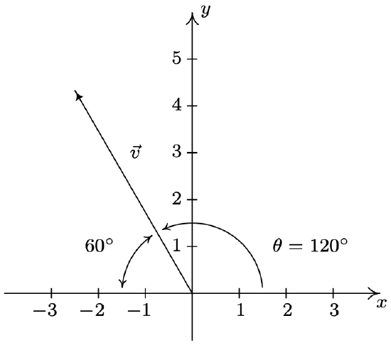
- Find the component form of the vector \(\vec{v}\) with \(\|\vec{v}\|=5\) so that when \(\vec{v}\) is plotted in standard position, it lies in Quadrant II and makes a \(60^{\circ}\) angle12 with the negative x-axis.
- For \(\vec{v}=\langle 3,-3 \sqrt{3}\rangle\), find \(\|\vec{v}\|\) and \(\theta\), \(0 \leq \theta<2 \pi\) so that \(\vec{v}=\|\vec{v}\|\langle\cos (\theta), \sin (\theta)\rangle\).
- For the vectors \(\vec{v}=\langle 3,4\rangle\) and \(\vec{w}=\langle 1,-2\rangle\), find the following.
- \(\hat{v}\)
- \(\|\vec{v}\|-2\|\vec{w}\|\)
- \(\|\vec{v}-2 \vec{w}\|\)
- \(\|\hat{w}\|\)
Solution
- We are told that \(\|\vec{v}\|=5\) and are given information about its direction, so we can use the formula \(\vec{v}=\|\vec{v}\| \hat{v}\) to get the component form of \(\vec{v}\). To determine \(\hat{v}\), we appeal to Definition 11.8. We are told that \(\vec{v}\) lies in Quadrant II and makes a \(60^{\circ}\) angle with the negative \(x\)-axis, so the polar form of the terminal point of \(\vec{v}\), when plotted in standard position is \(\left(5,120^{\circ}\right)\). (See the diagram below.) Thus \(\hat{v}=\left\langle\cos \left(120^{\circ}\right), \sin \left(120^{\circ}\right)\right\rangle=\left\langle-\frac{1}{2}, \frac{\sqrt{3}}{2}\right\rangle, \text { so } \vec{v}=\|\vec{v}\| \hat{v}=5\left\langle-\frac{1}{2}, \frac{\sqrt{3}}{2}\right\rangle=\left\langle-\frac{5}{2}, \frac{5 \sqrt{3}}{2}\right\rangle\).
- For \(\vec{v}=\langle 3,-3 \sqrt{3}\rangle\), we get \(\|\vec{v}\|=\sqrt{(3)^{2}+(-3 \sqrt{3})^{2}}=6\). In light of Definition 11.8, we can find the \(\theta\) we’re after by converting the point with rectangular coordinates \((3,-3 \sqrt{3})\) to polar form \((r, \theta)\) where \(r=\|\vec{v}\|>0\). From Section 11.4, we have \(\tan (\theta)=\frac{-3 \sqrt{3}}{3}=-\sqrt{3}\). Since \((3,-3 \sqrt{3})\) is a point in Quadrant IV, \(\theta\) is a Quadrant IV angle. Hence, we pick \(\theta=\frac{5 \pi}{3}\). We may check our answer by verifying \(\vec{v}=\langle 3,-3 \sqrt{3}\rangle=6\left\langle\cos \left(\frac{5 \pi}{3}\right), \sin \left(\frac{5 \pi}{3}\right)\right\rangle\).
-
- Since we are given the component form of \(\vec{v}\), we’ll use the formula \(\hat{v}=\left(\frac{1}{\|\vec{v}\|}\right) \vec{v}\). For \(\vec{v}=\langle 3,4\rangle\), we have \(\|\vec{v}\|=\sqrt{3^{2}+4^{2}}=\sqrt{25}=5\). Hence, \(\hat{v}=\frac{1}{5}\langle 3,4\rangle=\left\langle\frac{3}{5}, \frac{4}{5}\right\rangle\).
- We know from our work above that \(\|\vec{v}\|=5\), so to find \(\|\vec{v}\|-2\|\vec{w}\|\), we need only find \(\|\vec{w}\|\). Since \(\vec{w}=\langle 1,-2\rangle\), we get \(\|\vec{w}\|=\sqrt{1^{2}+(-2)^{2}}=\sqrt{5}\). Hence, \(\|\vec{v}\|-2\|\vec{w}\|=5-2 \sqrt{5}\).
- In the expression \(\|\vec{v}-2 \vec{w}\|\), notice that the arithmetic on the vectors comes first, then the magnitude. Hence, our first step is to find the component form of the vector \(\vec{v}-2 \vec{w}\). We get \(\vec{v}-2 \vec{w}=\langle 3,4\rangle-2\langle 1,-2\rangle=\langle 1,8\rangle\). Hence, \(\|\vec{v}-2 \vec{w}\|=\|\langle 1,8\rangle\|=\sqrt{1^{2}+8^{2}}=\sqrt{65}\).
- To find \(\|\hat{w}\|\), we first need \(\hat{w}\). Using the formula \(\hat{w}=\left(\frac{1}{\|\vec{w}\|}\right) \vec{w}\) along with \(\|\vec{w}\|=\sqrt{5}\), which we found the in the previous problem, we get \(\hat{w}=\frac{1}{\sqrt{5}}\langle 1,-2\rangle=\left\langle\frac{1}{\sqrt{5}},-\frac{2}{\sqrt{5}}\right\rangle=\left\langle\frac{\sqrt{5}}{5},-\frac{2 \sqrt{5}}{5}\right\rangle\). Hence, \(\|\hat{w}\|=\sqrt{\left(\frac{\sqrt{5}}{5}\right)^{2}+\left(-\frac{2 \sqrt{5}}{5}\right)^{2}}=\sqrt{\frac{5}{25}+\frac{20}{25}}=\sqrt{1}=1\).
The process exemplified by number 1 in Example 11.8.4 above by which we take information about the magnitude and direction of a vector and find the component form of a vector is called resolving a vector into its components. As an application of this process, we revisit Example 11.8.1 below.
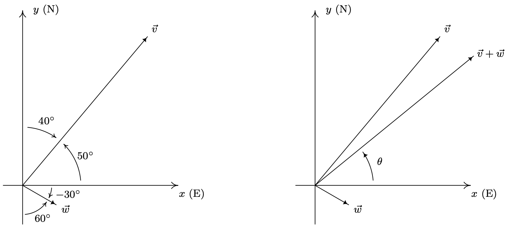
A plane leaves an airport with an airspeed of 175 miles per hour with bearing \(\mathrm{N} 40^{\circ} \mathrm{E}\). A 35 mile per hour wind is blowing at a bearing of \(\mathrm{S} 60^{\circ} \mathrm{E}\). Find the true speed of the plane, rounded to the nearest mile per hour, and the true bearing of the plane, rounded to the nearest degree.
Solution
We proceed as we did in Example 11.8.1 and let \(\vec{v}\) denote the plane’s velocity and \(\vec{w}\) denote the wind’s velocity, and set about determining \(\vec{v}+\vec{w}\). If we regard the airport as being at the origin, the positive \(y\)-axis acting as due north and the positive \(x\)-axis acting as due east, we see that the vectors \(\vec{v}\) and \(\vec{w}\) are in standard position and their directions correspond to the angles \(50^{\circ}\) and \(-30^{\circ}\), respectively. Hence, the component form of \(\vec{v}=175\left\langle\cos \left(50^{\circ}\right), \sin \left(50^{\circ}\right)\right\rangle=\left\langle 175 \cos \left(50^{\circ}\right), 175 \sin \left(50^{\circ}\right)\right\rangle\) and the component form of \(\vec{w}=\left\langle 35 \cos \left(-30^{\circ}\right), 35 \sin \left(-30^{\circ}\right)\right\rangle\). Since we have no convenient way to express the exact values of cosine and sine of \(50^{\circ}\), we leave both vectors in terms of cosines and sines.13 Adding corresponding components, we find the resultant vector \(\vec{v}+\vec{w}=\left\langle 175 \cos \left(50^{\circ}\right)+35 \cos \left(-30^{\circ}\right), 175 \sin \left(50^{\circ}\right)+35 \sin \left(-30^{\circ}\right)\right\rangle\). To find the ‘true’ speed of the plane, we compute the magnitude of this resultant vector \[\|\vec{v}+\vec{w}\|=\sqrt{\left(175 \cos \left(50^{\circ}\right)+35 \cos \left(-30^{\circ}\right)\right)^{2}+\left(175 \sin \left(50^{\circ}\right)+35 \sin \left(-30^{\circ}\right)\right)^{2}} \approx 184\nonumber\] Hence, the ‘true’ speed of the plane is approximately 184 miles per hour. To find the true bearing, we need to find the angle \(\theta\) which corresponds to the polar form \((r, \theta), r>0\), of the point \((x, y)=\left(175 \cos \left(50^{\circ}\right)+35 \cos \left(-30^{\circ}\right), 175 \sin \left(50^{\circ}\right)+35 \sin \left(-30^{\circ}\right)\right)\). Since both of these coordinates are positive,14 we know \(\theta\) is a Quadrant I angle, as depicted below. Furthermore, \[\tan (\theta)=\frac{y}{x}=\frac{175 \sin \left(50^{\circ}\right)+35 \sin \left(-30^{\circ}\right)}{175 \cos \left(50^{\circ}\right)+35 \cos \left(-30^{\circ}\right)},\nonumber\] so using the arctangent function, we get \(\theta \approx 39^{\circ}\). Since, for the purposes of bearing, we need the angle between \(\vec{v}+\vec{w}\) and the positive \(y\)-axis, we take the complement of \(\theta\) and find the ‘true’ bearing of the plane to be approximately \(\mathrm{N} 51^{\circ} \mathrm{E}\).
In part 3d of Example 11.8.4, we saw that \(\|\hat{w}\|=1\). Vectors with length 1 have a special name and are important in our further study of vectors.
Unit Vectors: Let \(\vec{v}\) be a vector. If \(\|\vec{v}\|=1\), we say that \(\vec{v}\) is a unit vector.
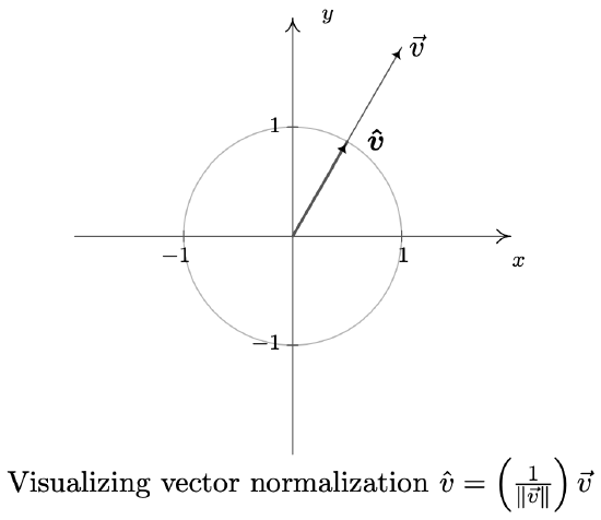
If \(\vec{v}\) is a unit vector, then necessarily, \(\vec{v}=\|\vec{v}\| \hat{v}=1 \cdot \hat{v}=\hat{v}\). Conversely, we leave it as an exercise15 to show that \(\hat{v}=\left(\frac{1}{\|\vec{v}\|}\right) \vec{v}\) is a unit vector for any nonzero vector \(\vec{v}\). In practice, if \(\vec{v}\) is a unit vector we write it as \(\vec{v}\) as opposed to \(\vec{v}\) because we have reserved the ‘ˆ’ notation for unit vectors. The process of multiplying a nonzero vector by the factor \(\frac{1}{\|\vec{v}\|}\) to produce a unit vector is called ‘normalizing the vector,’ and the resulting vector \(\vec{v}\) is called the ‘unit vector in the direction of \(\vec{v^{\prime}}\). The terminal points of unit vectors, when plotted in standard position, lie on the Unit Circle. (You should take the time to show this.) As a result, we visualize normalizing a nonzero vector \(\vec{v}\) as shrinking16 its terminal point, when plotted in standard position, back to the Unit Circle.
Of all of the unit vectors, two deserve special mention.
- The vector \(\hat{\imath}\) is defined by \(\hat{\imath}=\langle 1,0\rangle\)
- The vector \(\hat{\jmath}\) is defined by \(\hat{\imath}=\langle 0,1\rangle\)
We can think of the vector \(\hat{\imath}\) as representing the positive \(x\)-direction, while \(\hat{\jmath}\) represents the positive \(y\)-direction. We have the following ‘decomposition’ theorem.17
Let \(\vec{v}\) be a vector with component form \(\vec{v}=\left\langle v_{1}, v_{2}\right\rangle\). Then \(\vec{v}=v_{1} \hat{\imath}+v_{2} \hat{\jmath}\).
The proof of Theorem 11.21 is straightforward. Since \(\hat{\imath}=\langle 1,0\rangle\) and \(\hat{\jmath}=\langle 0,1\rangle\), we have from the definition of scalar multiplication and vector addition that
\(v_{1} \hat{\imath}+v_{2} \hat{\jmath}=v_{1}\langle 1,0\rangle+v_{2}\langle 0,1\rangle=\left\langle v_{1}, 0\right\rangle+\left\langle 0, v_{2}\right\rangle=\left\langle v_{1}, v_{2}\right\rangle=\vec{v}\)
Geometrically, the situation looks like this:
We conclude this section with a classic example which demonstrates how vectors are used to model forces. A ‘force’ is defined as a ‘push’ or a ‘pull.’ The intensity of the push or pull is the magnitude of the force, and is measured in Netwons (N) in the SI system or pounds (lbs.) in the English system.18 The following example uses all of the concepts in this section, and should be studied in great detail.
A 50 pound speaker is suspended from the ceiling by two support braces. If one of them makes a \(60^{\circ}\) angle with the ceiling and the other makes a \(30^{\circ}\) angle with the ceiling, what are the tensions on each of the supports?
Solution
We represent the problem schematically below and then provide the corresponding vector diagram.
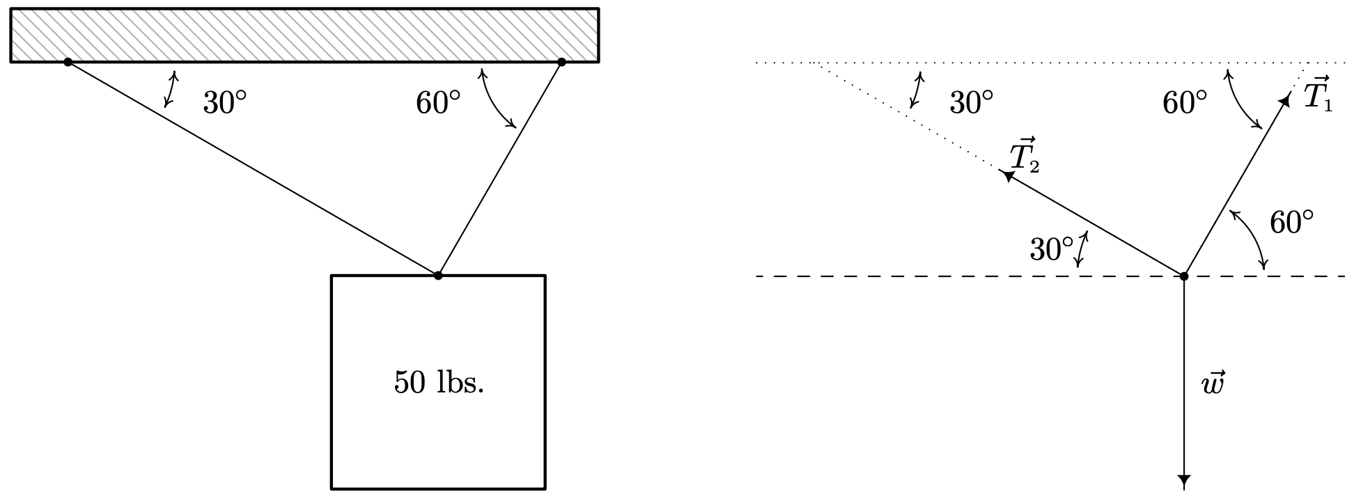
We have three forces acting on the speaker: the weight of the speaker, which we’ll call \(\vec{w}\), pulling the speaker directly downward, and the forces on the support rods, which we’ll call \(\vec{T}_{1}\) and \(\vec{T}_{2}\) (for ‘tensions’) acting upward at angles \(60^{\circ}\) and \(30^{\circ}\), respectively. We are looking for the tensions on the support, which are the magnitudes \(\left\|\vec{T}_{1}\right\|\) and \(\left\|\vec{T}_{2}\right\|\). In order for the speaker to remain stationary,19 we require \(\vec{w}+\overrightarrow{T_{1}}+\overrightarrow{T_{2}}=\overrightarrow{0}\). Viewing the common initial point of these vectors as the origin and the dashed line as the \(x\)-axis, we use Theorem 11.20 to get component representations for the three vectors involved. We can model the weight of the speaker as a vector pointing directly downwards with a magnitude of 50 pounds. That is, \(\|\vec{w}\|=50\) and \(\hat{w}=-\hat{\jmath}=\langle 0,-1\rangle\). Hence, \(\vec{w}=50\langle 0,-1\rangle=\langle 0,-50\rangle\). For the force in the first support, we get \[\begin{aligned}
\vec{T}_{1} &=\left\|\vec{T}_{1}\right\|\left\langle\cos \left(60^{\circ}\right), \sin \left(60^{\circ}\right)\right\rangle \\ &=\left\langle\frac{\left\|\vec{T}_{1}\right\|}{2}, \frac{\left\|\vec{T}_{1}\right\| \sqrt{3}}{2}\right\rangle \end{aligned}\nonumber\] For the second support, we note that the angle \(30^{\circ}\) is measured from the negative \(x\)-axis, so the angle needed to write \(\overrightarrow{T_{2}}\) in component form is \(150^{\circ}\). Hence \[\begin{aligned} \vec{T}_{2} &=\left\|\vec{T}_{2}\right\|\left\langle\cos \left(150^{\circ}\right), \sin \left(150^{\circ}\right)\right\rangle \\ &=\left\langle-\frac{\left\|\vec{T}_{2}\right\| \sqrt{3}}{2}, \frac{\left\|\vec{T}_{2}\right\|}{2}\right\rangle
\end{aligned}\] The requirement \(\vec{w}+\vec{T}_{1}+\vec{T}_{2}=\overrightarrow{0}\) gives us this vector equation. \[\begin{array}{rrl}
&\vec{w}+\vec{T}_{1}+\vec{T}_{2}&=&\overrightarrow{0}\\ &\langle 0,-50\rangle+\left\langle\frac{\left\|\vec{T}_{1}\right\|}{2}, \frac{\left\|\vec{T}_{1}\right\| \sqrt{3}}{2}\right\rangle+\left\langle-\frac{\left\|\vec{T}_{2}\right\| \sqrt{3}}{2}, \frac{\left\|\vec{T}_{2}\right\|}{2}\right\rangle&=&\langle 0,0\rangle\\ &\left\langle\frac{\left\|\vec{T}_{1}\right\|}{2}-\frac{\left\|\vec{T}_{2}\right\| \sqrt{3}}{2}, \frac{\left\|\vec{T}_{1}\right\| \sqrt{3}}{2}+\frac{\left\|\vec{T}_{2}\right\|}{2}-50\right\rangle&=&\langle 0,0\rangle \end{array}\nonumber\] Equating the corresponding components of the vectors on each side, we get a system of linear equations in the variables \(\left\|\overrightarrow{T_{1}}\right\|\) and \(\left\|\vec{T}_{2}\right\|\). \[\left\{\begin{array}{l} (E 1) \quad \frac{\left\|\vec{T}_{1}\right\|}{2}-\frac{\left\|\vec{T}_{2}\right\| \sqrt{3}}{2}&=0 \\ (E 2) \frac{\left\|\vec{T}_{1}\right\| \sqrt{3}}{2}+\frac{\left\|\vec{T}_{2}\right\|}{2}-50&=0 \end{array}\right.\nonumber\] From \((E 1)\), we get \(\left\|\vec{T}_{1}\right\|=\left\|\vec{T}_{2}\right\| \sqrt{3}\). Substituting that into \((E 2)\) gives \(\frac{\left(\left\|\overrightarrow{T_{2}}\right\| \sqrt{3}\right) \sqrt{3}}{2}+\frac{\left\|\vec{T}_{2}\right\|}{2}-50=0\) which yields \(2\left\|\vec{T}_{2}\right\|-50=0\). Hence, \(\left\|\vec{T}_{2}\right\|=25\) pounds and \(\left\|\vec{T}_{1}\right\|=\left\|\vec{T}_{2}\right\| \sqrt{3}=25 \sqrt{3}\) pounds.
1 The word ‘vector’ comes from the Latin vehere meaning ‘to convey’ or ‘to carry.’
2 Other textbook authors use bold vectors such as \(\boldsymbol{v}\). We find that writing in bold font on the chalkboard is inconvenient at best, so we have chosen the ‘arrow’ notation.
3 If this idea of ‘over’ and ‘up’ seems familiar, it should. The slope of the line segment containing \(\vec{v}\) is \(\frac{4}{3}\).
4 If necessary, review page 905 and Section 11.3.
5 That is, the speed of the plane relative to the air around it. If there were no wind, plane’s airspeed would be the same as its speed as observed from the ground. How does wind affect this? Keep reading!
6 See Section 10.1.1, for instance.
7 Or, since our given angle, \(100^{\circ}\), is obtuse, we could use the Law of Sines without any ambiguity here.
8 Adding vectors ‘component-wise’ should seem hauntingly familiar. Compare this with how matrix addition was defined in section 8.3. In fact, in more advanced courses such as Linear Algebra, vectors are defined as \(1 \times n\) or \(n \times 1\) matrices, depending on the situation.
9 The interested reader is encouraged to compare Theorem 11.18 and the ensuing discussion with Theorem 8.3 in Section 8.3 and the discussion there.
10 If this all looks familiar, it should. The interested reader is invited to compare Definition 11.8 to Definition 11.2 in Section 11.7.
11 Of course, to go from \(\vec{v}=\|\vec{v}\| \hat{v}\) to \(\hat{v}=\left(\frac{1}{\|\vec{v}\|}\right) \vec{v}\), we are essentially ‘dividing both sides’ of the equation by the scalar \(\|\vec{v}\|\). The authors encourage the reader, however, to work out the details carefully to gain an appreciation of the properties in play.
12 Due to the utility of vectors in ‘real-world’ applications, we will usually use degree measure for the angle when giving the vector’s direction. However, since Carl doesn’t want you to forget about radians, he’s made sure there are examples and exercises which use them.
13 Keeping things ‘calculator’ friendly, for once!
14 Yes, a calculator approximation is the quickest way to see this, but you can also use good old-fashioned inequalities and the fact that \(45^{\circ} \leq 50^{\circ} \leq 60^{\circ}\).
15 One proof uses the properties of scalar multiplication and magnitude. If \(\vec{v} \neq \overrightarrow{0}\), consider \(\|\hat{v}\|=\left\|\left(\frac{1}{\|\vec{v}\|}\right) \vec{v}\right\|\). Use the fact that \(\|\vec{v}\| \geq 0\) is a scalar and consider factoring.
16 . . . if \(\|\vec{v}\|>1\). . .
17 We will see a generalization of Theorem 11.21 in Section 11.9. Stay tuned!
18 See also Section 11.1.1.
19 This is the criteria for ‘static equilbrium’.