1.4: Circles and Angles in the Rectangular Coordinate System

Note to the Instructor (click to expand) Up to this point, all of your instruction should have omitted the Cartesian coordinate system and equations depicting solutions on that plane. We now glue our beloved coordinate system to the Geometry reviewed up to point. Much of the content here cannot be done without mastering the previous sections. To succeed in this section, you'll need to use some skills from previous courses. While you should already know them, this is the first time they've been required. You can review these skills in CRC's Corequisite Codex. If you have a support class, it might cover some, but not all, of these topics. Prerequisite Skills and Support Topics (click to expand) Sets and Numbers Sets of Numbers: The set of integers is needed from this point forward in Trigonometry. Solving Equations Solving Quadratic Equations: This skill is required when finding coordinates of points on a circle, such as in Example 6 where solving for \(y\) in \( (-1)^2 + y^2 = 4 \) is necessary. Graphs The Cartesian Coordinate System and the Quadrants: This section is built upon the coordinate plane, where concepts like the Distance Formula, circles, and angles in standard position are defined. Ordered Pairs and Graphing Relations by Point-Plotting: This skill is used to locate points, graph circles, and understand the position of angles in the plane. The following is a list of learning objectives for this section. Learning Objectives (click to expand) Compute the distance between two points on the Cartesian plane. Verify a point lies on the unit circle. Graph a circle given its equation. Determine in which quadrant an angle in standard position terminates. Sketch an angle in standard position. Find an angle coterminal with a given angle.

Hawk A.I. Section-Specific Tutor To access the Hawk A.I. Tutor, you will need to be logged into your campus Gmail account.

The Distance Formula

Matt is hiking in the Santa Monica mountains. He would like to know the distance from the Sycamore Canyon trailhead, located at \(12-\mathrm{C}\) on his map, to the Coyote Trail junction, located at \(8-\mathrm{F}\), as shown below.

Figure \( \PageIndex{ 1 } \)

Each interval on the map represents one kilometer. Matt remembers the Pythagorean Theorem and uses the map coordinates to label the sides of a right triangle. The distance he wants is the hypotenuse of the triangle, so\[\begin{array}{rrcl}
& d^2 & = & 4^2+3^2 \\
\implies & d^2 & = & 16 + 9 \\
\implies & d^2 & = & 25 \\
\implies & d & = & \sqrt{25} \\
\implies & d & = & 5 \\
\end{array} \nonumber \]The straight-line distance to Coyote junction is about 5 kilometers. The formula for the distance between two points is obtained similarly.

We first label a right triangle with points \(P_1\) and \(P_2\) on opposite ends of the hypotenuse (see Figure \( \PageIndex{ 2 } \)). The sides of the triangle have lengths \(|x_2 - x_1|\) and \(|y_2 - y_1|\). We can use the Pythagorean Theorem to calculate the distance between \(P_1\) and \(P_2\): \(d^2 = (x_2-x_1)^2 + (y_2 - y_1)^2\).

Figure \( \PageIndex{ 2 } \)

Taking the (positive) square root of each side of this equation gives us the Distance Formula.

Theorem: Distance Formula

The distance \(d\) between two points \(P_1\left(x_1, y_1\right)\) and \(P_2\left(x_2, y_2\right)\) is\[d=\sqrt{\left(x_2-x_1\right)^2+\left(y_2-y_1\right)^2}. \nonumber\]

Example \( \PageIndex{ 1 } \)

Find the distance between (2, −1) and (4, 3).

Solution

We substitute \((2,-1)\) for \(\left(x_1, y_1\right)\) and \((4,3)\) for \(\left(x_2, y_2\right)\) in the Distance Formula to obtain

Figure \( \PageIndex{ 3 } \)

\[\begin{array}{rrrclcl}
& & d &=&\sqrt{\left(x_2-x_1\right)^2+\left(y_2-y_1\right)^2} & \quad & \left( \text{Distance Formula} \right) \\
\scriptscriptstyle\xcancel{\mathrm{Arithmetic}} \to \mathrm{Algebra}&\implies & & = & \sqrt{(4-2)^2+[3-(-1)]^2} & \quad & \left( \text{substitution} \right)\\
\scriptscriptstyle\mathrm{Arithmetic}&\implies & & = & \sqrt{2^2+4^2} & \quad & \left( \text{addition and subtraction} \right) \\
\scriptscriptstyle\mathrm{Arithmetic}&\implies & & = & \sqrt{4 + 16} & \quad & \left( \text{applying powers} \right) \\
\scriptscriptstyle\mathrm{Arithmetic}&\implies & & = & \sqrt{20} & \quad & \left( \text{addition} \right) \\
\scriptscriptstyle\mathrm{Arithmetic}&\implies & & = & 2 \sqrt{5} & \quad & \left( \text{simplify the radical} \right)
\end{array} \nonumber \]The exact value of the distance, shown at right, is \(2 \sqrt{5}\) units. We obtain the same answer if we use \((4,3)\) for \(P_1\) and \((2,-1)\) for \(P_2\):\[ \begin{array}{rcl}
d & = & \sqrt{(2-4)^2+[(-1)-3]^2} \\[6pt]
& = & \sqrt{4+16} \\[6pt]
& = & \sqrt{20} \\[6pt]
& = & 2 \sqrt{5} \\[6pt]
\end{array} \nonumber \]We can use a calculator to obtain an approximation for this value and find \(2 \sqrt{5} \approx 2(2.236)=4.472 \).

Critical Mistake

In Example \( \PageIndex{ 1 } \), the radical \(\sqrt{4+16}\) cannot be simplified to \(\sqrt{4}+\sqrt{16}\). (Do you remember why not?)

Checkpoint \( \PageIndex{ 1 } \)

1. Find the distance between the points (−5, 3) and (3, −9).
2. Plot the points on a Cartesian coordinate system and show how the Pythagorean Theorem is used to calculate the distance.

Answers

1. \(4\sqrt{13}\)
2. The points (−5, 3) and (3, −9) are two vertices of a right triangle with one horizontal leg of length 8 and one vertical leg of length 12. The distance between (−5, 3) and (3, −9) is the hypotenuse \(c\).
   

Equation for a Circle

The Distance Formula is required for us to find the equation of a circle.

Theorem: Equation of a Circle Centered at the Origin

The equation for a circle of radius \(r\) centered at the origin is\[x^2 + y^2 = r^2. \nonumber \]

Proof

Consider a circle of radius \( r \) centered at the origin, as shown in the following figure.

The circle of radius \( r \) centered at the origin

The distance from the origin to any point \(P(x, y)\) on the circle is \(r\). Therefore, by the Distance Formula,\[\sqrt{(x-0)^2+(y-0)^2} = r\nonumber \]or, squaring both sides,\[(x-0)^2 + (y-0)^2 = r^2. \nonumber \]Because every point on the circle must satisfy this equation, we have found an equation for the circle.

Example \( \PageIndex{ 2 } \)

Find two points on the circle \(x^2+y^2=4\) with an \(x\)-coordinate of \(-1\).

Solution

We substitute \(x=-1\) into the equation for the circle and solve for \(y\).\[\begin{array}{rrrclcl}
\scriptscriptstyle\xcancel{\mathrm{Arithmetic}} \to \mathrm{Algebra} & \implies & (-1)^2+y^2 & = & 4 & \quad & \left( \text{substitution} \right) \\
\scriptscriptstyle\mathrm{Arithmetic} & \implies & 1 + y^2 & = & 4 & \quad & \left( \text{applying the power} \right) \\
\scriptscriptstyle\xcancel{\mathrm{Arithmetic}} \to \mathrm{Algebra} & \implies & y^2 & = & 3 & \quad & \left( \text{subtract }1\text{ from both sides} \right) \\
\scriptscriptstyle\xcancel{\mathrm{Arithmetic}} \to \mathrm{Algebra} & \implies & y & = & \pm\sqrt{3} & \quad & \left( \text{Extraction of Roots} \right) \\
\end{array}\nonumber \]

Figure \( \PageIndex{ 4 } \)

The points are \((-1,\sqrt{3})\) and \((-1,\sqrt{3})\), as shown at right. Note that \(\sqrt{3} \approx 1.732\).

Checkpoint \( \PageIndex{ 2 } \)

Find the coordinates of two points on the circle \(x^2 + y^2 = 1\) with \(y\)-coordinate \(\dfrac{1}{2}\).

Answer

\(\left(\frac{\sqrt{3}}{2}, \frac{1}{2}\right),\left(-\frac{\sqrt{3}}{2}, \frac{1}{2}\right)\)

The circle in Checkpoint \( \PageIndex{ 2} \) holds a special place in Trigonometry.

Definition: Unit Circle

The circle centered at the origin and having radius 1, is called the unit circle. The unit circle has equation\[ x^2 + y^2 = 1. \nonumber \]

While the definition of the unit circle is only mentioned in passing here, it will become one of the foundational pieces of Trigonometry. We will revisit this later.

Later in this course, we will need to work with circles that do not have centers at the origin.

Theorem: Equation of a Circle Centered Off-Origin

The equation for a circle of radius \(r\) centered at the point \( \left( h,k \right) \) is\[(x - h)^2 + (y - k)^2 = r^2. \nonumber \]This is also know as the standard form of the equation of a circle.

Proof

Consider a circle of radius \( r \) centered at the point \( \left( h,k \right) \), as shown in the following figure.

A circle of radius \( r \) centered at the point \( \left( h,k \right) \)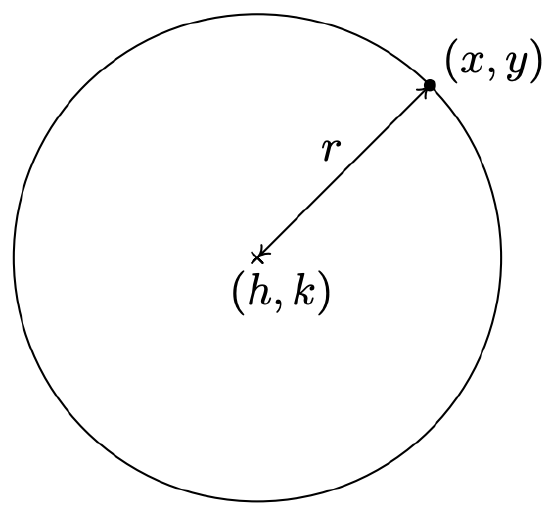

Since this is a circle of radius \( r \), the point \((x,y)\) is on the circle if and only if its distance to \((h,k)\) is \(r\). By the Distance Formula, this means\[r = \sqrt{(x - h)^2 + (y-k)^2}.\nonumber\]By squaring both sides of this equation, we get\[ r^2 = (x - h)^2 + (y - k)^2. \nonumber \]

Example \( \PageIndex{3} \)

Write the standard equation of the circle with center \((-2,3)\) and radius \(5\).

Solution

Here, \((h,k) = (-2,3)\) and \(r = 5\), so we get\[\begin{array}{rrcl}
& (x-(-2))^2+(y-3)^2 & = & (5)^2 \\
\implies & (x+2)^2+(y-3)^2 & = & 25 \\
\end{array}\nonumber\]

Checkpoint \( \PageIndex{3} \)

Graph \((x+2)^2+(y-1)^2 = 4\). Find the center and radius.

Answer

From the standard form of a circle we have that \(x + 2\) is \(x-h\), so \(h = -2\) and \(y - 1\) is \(y - k\) so \(k = 1\). This tells us that our center is \((-2,1)\). Furthermore, \(r^2 = 4\), so \(r = 2\). Thus we have a circle centered at \((-2,1)\) with a radius of \(2\). Graphing gives us

Figure \( \PageIndex{ 5 } \)

Angles in the Cartesian Coordinate System

Now that we have reacquainted ourselves with angles, circles, and the Cartesian coordinate system, the next natural evolution toward Trigonometry is introducing angles to the Cartesian coordinate plane. Before we begin, however, it will be instrumental in this course to divide the Cartesian coordinate system into four sections, called quadrants.

Definition: Quadrants

In the Cartesian coordinate system, the section of the plane where

• \( x \) and \( y \) are both positive is called Quadrant I (QI),
• \( x < 0 \) and \( y > 0 \) is called Quadrant II (QII),
• \( x \) and \( y \) are both negative is called Quadrant III (QIII), and
• \( x > 0 \) and \( y < 0 \) is called Quadrant IV (QIV).

The four quadrants of the Cartesian coordinate system

Knowing this definition and understanding how the signs of \( x \) and \( y \) relate to these quadrants will be critical as we move forward.

Angles in Standard Position

In general, and without worrying about a coordinate system, the degree measure of an angle depends only on the fraction of a whole rotation between its sides, not on the angle's location or position. To compare and analyze angles, we place them in standard position.

Definition: Standard Position of an Angle

An angle is said to be in standard position if the vertex of the angle is at the origin and the initial side of the angle is on the positive \( x \)-axis.

Figure \( \PageIndex{ 6 } \) below shows several angles moved into standard position.

Figure \( \PageIndex{ 6 } \): Angles in nonstandard position (top row) and their equivalent angles in standard position (bottom row)

The \( 320^{ \circ } \) in Figure \( \PageIndex{ 6 } \) has its terminal side in quadrant IV. We denote this as \( 320^{ \circ } \in \mathrm{QIV}\). Likewise, the remaining angles in Figure \( \PageIndex{ 6 } \) are listed as \( 240^{ \circ } \in \mathrm{QIII} \), \( 130^{ \circ } \in \mathrm{QII} \), and \( 55^{ \circ } \in \mathrm{QI} \).

Example \( \PageIndex{ 4 } \)

Find the degree measure of each angle shown below, state the quadrant where the angle terminates, and sketch the angle in standard position.

Figure \( \PageIndex{ 7 } \)

Solutions

1. The angle \(\alpha\) is one-fifth of a complete revolution, or\[\dfrac{1}{5}(360^{\circ}) = 72^{\circ}.\nonumber \]In standard position, \( \alpha = 72^{ \circ } \in \mathrm{QI} \), as shown in Figure \( \PageIndex{ 8(a) } \) below.

   Figure \( \PageIndex{ 8 } \)

   

2. The angle \(\beta\) is \(\dfrac{11}{12}\) of a complete revolution, or\[\dfrac{11}{12}(360^{\circ}) = 330^{\circ}.\nonumber \]In standard position, \( \beta = 330^{ \circ } \in \mathrm{QIV} \). (See Figure \( \PageIndex{ 8(b) } \).)

Checkpoint \( \PageIndex{ 4 } \)

Find the degree measure of each angle below, sketch the angle in standard position, and state the quadrant in which the angle terminates.

Figure \( \PageIndex{ 9 } \)

Answers

1. \(\theta = 120^{\circ} \in \mathrm{QII}\)

   Figure \( \PageIndex{ 10 } \)

   

2. \(\alpha = 250^{ \circ } - 180^{ \circ } = 70^{\circ} \in \mathrm{QI}\)

   Figure \( \PageIndex{ 11 } \)

   

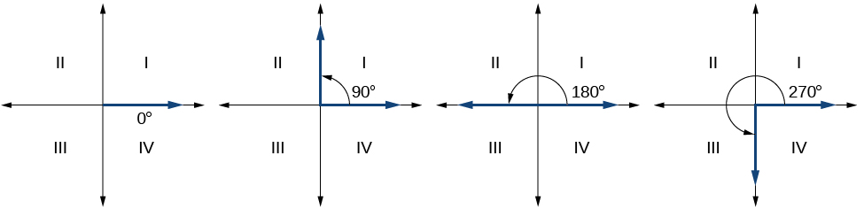
Quadrantal Angles

Now that we are acquainted with angles in standard position, it's time we start classifying these angles by type. First up are the quadrantal angles.

Definition: Quadrantal Angle

An angle in standard position having terminal side on an axis is called a quadrantal angle.

For example, \( 270^{ \circ } \) has a terminal side on the negative \( y \)-axis. Therefore, we would call \( 270^{ \circ } \) a quadrantal angle. Figure \( \PageIndex{ 12 } \) illustrates a few quadrantal angles; however, as we will learn shortly, there are infinite quadrantal angles.

Figure \( \PageIndex{ 12 } \): Some quadrantal angles

Negative Angles

Aligning with what we said earlier in this textbook, an angle is positive if it opens counterclockwise. If an angle opens clockwise, the angle is considered negative. For example, Figure \( \PageIndex{ 13 } \) shows the angle \( \alpha = -135^{ \circ } \), which terminates in \( \mathrm{QIII} \).

Figure \( \PageIndex{ 13 } \): A negative angle

Graphing positive and negative angles in standard position will be a critical skill in Trigonometry.

Coterminal Angles

Because \(360^{\circ}\) represents one complete revolution, we can add or subtract a multiple of \(360^{\circ}\) to any angle and the terminal side of the resulting angle will arrive at the same position. For example, the angles \(70^{\circ}\) and \(430^{\circ}\) have the same terminal side because \(430^{\circ}=70^{\circ}+360^{\circ}\). Such angles are called coterminal.

Definition: Coterminal Angles

Angles in standard position that share a terminal side are called coterminal angles.

The angle \(790^{\circ}\) is also coterminal with \(70^{\circ}\), because \(790^{\circ}=70^{\circ}+2\left(360^{\circ}\right)\) (see Figure \( \PageIndex{ 14 } \) below).

Figure \( \PageIndex{ 14 } \): Graphical representations of coterminal angles

Coterminal angles need not be positive. For example, we could have been given \( \alpha = 140^{ \circ } \) and chosen to subtract \( 360^{ \circ } \) to get the coterminal angle \( -220^{ \circ } \) as shown in Figure \( \PageIndex{ 15 } \).

Figure \( \PageIndex{ 15 } \)

In fact, we could denote all angles coterminal to \( \alpha = 140^{ \circ } \) using the notation\[ 140^{ \circ } + 360^{ \circ }k, \text{ where } k \in \mathbb{Z}. \nonumber \]The symbol, \( \mathbb{Z} \), denotes the set of all integers (the set of numbers \( \ldots, -3, -2, -1, 0, 1, 2, 3, \ldots \)). This notation gets used frequently in Mathematics from this point forward, so it is best to get used to it quickly.

Theorem: Cotermial Angle Formula

All angles coterminal to the angle \( \alpha \) (in standard position) have the form\[ \alpha + 360^{ \circ } k, \text{ where } k \in \mathbb{Z}. \nonumber \]

Previously, we mentioned that the angles illustrated in Figure \( \PageIndex{ 12 } \) were only a "few quadrantal angles," implying there were more than what we listed. This was because, for example, given the quadrantal angle \( 90^{ \circ } \), we could generate an infinite number of other quadrantal angles with the same terminal side by considering\[ 90^{ \circ } + 360^{ \circ }k, \text{ where } k \in \mathbb{Z}. \nonumber \]Moreover, since the quadrantal angles only differ from each other by \( 90^{ \circ } \), we could generate all quadrantal angles with the single statement\[ 0^{ \circ } + 90^{ \circ }k, \text{ where } k \in \mathbb{Z}. \nonumber \]There is no need for the \( 0^{ \circ } \) angle in that formula, so we could shorten it up to just\[ 90^{ \circ }k, \text{ where } k \in \mathbb{Z}. \nonumber \]

Example \( \PageIndex{5} \)

Graph each of the angles below in standard position and classify them according to where their terminal side lies. Find three coterminal angles, at least one of which is positive and one of which is negative.

1. \(\alpha = 60^{\circ}\)
2. \(\beta = -225^{\circ}\)
3. \(\gamma = 540^{\circ}\)
4. \(\phi = -750^{\circ}\)

Solutions

1. To graph \(\alpha = 60^{\circ}\), we draw an angle with its initial side on the positive \(x\)-axis and rotate counter-clockwise \(\frac{60^{\circ}}{360^{\circ}} = \frac{1}{6}\) of a revolution. We see that \(\alpha\) is a Quadrant I angle. To find coterminal angles, we look for angles \(\theta\) of the form \(\theta = \alpha + 360^{\circ} \cdot k\), for some integer \(k\). When \(k = 1\), we get \(\theta = 60^{\circ} + 360^{\circ} = 420^{\circ}\). Substituting \(k = -1\) gives \(\theta = 60^{\circ} - 360^{\circ} = -300^{\circ}\). Finally, if we let \(k = 2\), we get \(\theta = 60^{\circ} + 720^{\circ} = 780^{\circ}\).
2. Since \(\beta = - 225^{\circ}\) is negative, we start at the positive \(x\)-axis and rotate clockwise \(\frac{225^{\circ}}{360^{\circ}} = \frac{5}{8}\) of a revolution. We see that \(\beta\) is a Quadrant II angle. To find coterminal angles, we proceed as before and compute \(\theta = -225^{\circ} + 360^{\circ} \cdot k\) for integer values of \(k\). We find \(135^{\circ}\), \(-585^{\circ}\) and \(495^{\circ}\) are all coterminal with \(-225^{\circ}\).

   Figure \( \PageIndex{ 16 } \)

   

3. Since \(\gamma = 540^{\circ}\) is positive, we rotate counter-clockwise from the positive \(x\)-axis. One full revolution accounts for \(360^{\circ}\), with \(180^{\circ}\), or \(\frac{1}{2}\) of a revolution remaining. Since the terminal side of \(\gamma\) lies on the negative \(x\)-axis, \(\gamma\) is a quadrantal angle. All angles coterminal with \(\gamma\) are of the form \(\theta = 540^{\circ} + 360^{\circ} \cdot k\), where \(k\) is an integer. Working through the arithmetic, we find three such angles: \(180^{\circ}\), \(-180^{\circ}\) and \(900^{\circ}\).
4. The Greek letter \(\phi\) is pronounced "fee" or "fie," and since \(\phi\) is negative, we begin our rotation clockwise from the positive \(x\)-axis. Two full revolutions account for \(720^{\circ}\), with just \(30^{\circ}\) or \(\frac{1}{12}\) of a revolution to go. We find that \(\phi\) is a Quadrant IV angle. To find coterminal angles, we compute \(\theta = -750^{\circ} + 360^{\circ} \cdot k\) for a few integers \(k\) and obtain \(-390^{\circ}\), \(-30^{\circ}\) and \(330^{\circ}\).

   Figure \( \PageIndex{ 17 } \)

   

Checkpoint \( \PageIndex{ 5 } \)

Find two angles coterminal with \(102^{\circ}\), one positive and one negative.

Answer

\(462^{\circ},-258^{\circ}\)