
1.4: Arc Length of a Curve and Surface Area
- Page ID
- 128814

\( \newcommand{\vecs}[1]{\overset { \scriptstyle \rightharpoonup} {\mathbf{#1}} } \)
\( \newcommand{\vecd}[1]{\overset{-\!-\!\rightharpoonup}{\vphantom{a}\smash {#1}}} \)
\( \newcommand{\id}{\mathrm{id}}\) \( \newcommand{\Span}{\mathrm{span}}\)
( \newcommand{\kernel}{\mathrm{null}\,}\) \( \newcommand{\range}{\mathrm{range}\,}\)
\( \newcommand{\RealPart}{\mathrm{Re}}\) \( \newcommand{\ImaginaryPart}{\mathrm{Im}}\)
\( \newcommand{\Argument}{\mathrm{Arg}}\) \( \newcommand{\norm}[1]{\| #1 \|}\)
\( \newcommand{\inner}[2]{\langle #1, #2 \rangle}\)
\( \newcommand{\Span}{\mathrm{span}}\)
\( \newcommand{\id}{\mathrm{id}}\)
\( \newcommand{\Span}{\mathrm{span}}\)
\( \newcommand{\kernel}{\mathrm{null}\,}\)
\( \newcommand{\range}{\mathrm{range}\,}\)
\( \newcommand{\RealPart}{\mathrm{Re}}\)
\( \newcommand{\ImaginaryPart}{\mathrm{Im}}\)
\( \newcommand{\Argument}{\mathrm{Arg}}\)
\( \newcommand{\norm}[1]{\| #1 \|}\)
\( \newcommand{\inner}[2]{\langle #1, #2 \rangle}\)
\( \newcommand{\Span}{\mathrm{span}}\) \( \newcommand{\AA}{\unicode[.8,0]{x212B}}\)
\( \newcommand{\vectorA}[1]{\vec{#1}} % arrow\)
\( \newcommand{\vectorAt}[1]{\vec{\text{#1}}} % arrow\)
\( \newcommand{\vectorB}[1]{\overset { \scriptstyle \rightharpoonup} {\mathbf{#1}} } \)
\( \newcommand{\vectorC}[1]{\textbf{#1}} \)
\( \newcommand{\vectorD}[1]{\overrightarrow{#1}} \)
\( \newcommand{\vectorDt}[1]{\overrightarrow{\text{#1}}} \)
\( \newcommand{\vectE}[1]{\overset{-\!-\!\rightharpoonup}{\vphantom{a}\smash{\mathbf {#1}}}} \)
\( \newcommand{\vecs}[1]{\overset { \scriptstyle \rightharpoonup} {\mathbf{#1}} } \)
\( \newcommand{\vecd}[1]{\overset{-\!-\!\rightharpoonup}{\vphantom{a}\smash {#1}}} \)
\(\newcommand{\avec}{\mathbf a}\) \(\newcommand{\bvec}{\mathbf b}\) \(\newcommand{\cvec}{\mathbf c}\) \(\newcommand{\dvec}{\mathbf d}\) \(\newcommand{\dtil}{\widetilde{\mathbf d}}\) \(\newcommand{\evec}{\mathbf e}\) \(\newcommand{\fvec}{\mathbf f}\) \(\newcommand{\nvec}{\mathbf n}\) \(\newcommand{\pvec}{\mathbf p}\) \(\newcommand{\qvec}{\mathbf q}\) \(\newcommand{\svec}{\mathbf s}\) \(\newcommand{\tvec}{\mathbf t}\) \(\newcommand{\uvec}{\mathbf u}\) \(\newcommand{\vvec}{\mathbf v}\) \(\newcommand{\wvec}{\mathbf w}\) \(\newcommand{\xvec}{\mathbf x}\) \(\newcommand{\yvec}{\mathbf y}\) \(\newcommand{\zvec}{\mathbf z}\) \(\newcommand{\rvec}{\mathbf r}\) \(\newcommand{\mvec}{\mathbf m}\) \(\newcommand{\zerovec}{\mathbf 0}\) \(\newcommand{\onevec}{\mathbf 1}\) \(\newcommand{\real}{\mathbb R}\) \(\newcommand{\twovec}[2]{\left[\begin{array}{r}#1 \\ #2 \end{array}\right]}\) \(\newcommand{\ctwovec}[2]{\left[\begin{array}{c}#1 \\ #2 \end{array}\right]}\) \(\newcommand{\threevec}[3]{\left[\begin{array}{r}#1 \\ #2 \\ #3 \end{array}\right]}\) \(\newcommand{\cthreevec}[3]{\left[\begin{array}{c}#1 \\ #2 \\ #3 \end{array}\right]}\) \(\newcommand{\fourvec}[4]{\left[\begin{array}{r}#1 \\ #2 \\ #3 \\ #4 \end{array}\right]}\) \(\newcommand{\cfourvec}[4]{\left[\begin{array}{c}#1 \\ #2 \\ #3 \\ #4 \end{array}\right]}\) \(\newcommand{\fivevec}[5]{\left[\begin{array}{r}#1 \\ #2 \\ #3 \\ #4 \\ #5 \\ \end{array}\right]}\) \(\newcommand{\cfivevec}[5]{\left[\begin{array}{c}#1 \\ #2 \\ #3 \\ #4 \\ #5 \\ \end{array}\right]}\) \(\newcommand{\mattwo}[4]{\left[\begin{array}{rr}#1 \amp #2 \\ #3 \amp #4 \\ \end{array}\right]}\) \(\newcommand{\laspan}[1]{\text{Span}\{#1\}}\) \(\newcommand{\bcal}{\cal B}\) \(\newcommand{\ccal}{\cal C}\) \(\newcommand{\scal}{\cal S}\) \(\newcommand{\wcal}{\cal W}\) \(\newcommand{\ecal}{\cal E}\) \(\newcommand{\coords}[2]{\left\{#1\right\}_{#2}}\) \(\newcommand{\gray}[1]{\color{gray}{#1}}\) \(\newcommand{\lgray}[1]{\color{lightgray}{#1}}\) \(\newcommand{\rank}{\operatorname{rank}}\) \(\newcommand{\row}{\text{Row}}\) \(\newcommand{\col}{\text{Col}}\) \(\renewcommand{\row}{\text{Row}}\) \(\newcommand{\nul}{\text{Nul}}\) \(\newcommand{\var}{\text{Var}}\) \(\newcommand{\corr}{\text{corr}}\) \(\newcommand{\len}[1]{\left|#1\right|}\) \(\newcommand{\bbar}{\overline{\bvec}}\) \(\newcommand{\bhat}{\widehat{\bvec}}\) \(\newcommand{\bperp}{\bvec^\perp}\) \(\newcommand{\xhat}{\widehat{\xvec}}\) \(\newcommand{\vhat}{\widehat{\vvec}}\) \(\newcommand{\uhat}{\widehat{\uvec}}\) \(\newcommand{\what}{\widehat{\wvec}}\) \(\newcommand{\Sighat}{\widehat{\Sigma}}\) \(\newcommand{\lt}{<}\) \(\newcommand{\gt}{>}\) \(\newcommand{\amp}{&}\) \(\definecolor{fillinmathshade}{gray}{0.9}\)- Determine the length of a curve, \(y=f(x)\), between two points.
- Determine the length of a curve, \(x=g(y)\), between two points.
- Find the surface area of a solid of revolution.
In this section, we use definite integrals to find the arc length of a curve. We can think of arc length as the distance you would travel if you were walking along the path of the curve. Many real-world applications involve arc length. If a rocket is launched along a parabolic path, we might want to know how far the rocket travels. Or, if a curve on a map represents a road, we might want to know how far we have to drive to reach our destination.
We begin by calculating the arc length of curves defined as functions of \( x \), then we examine the same process for curves defined as functions of \( y \).1 The techniques we use to find arc length can be extended to find the surface area of a surface of revolution, and we close the section with an examination of this concept.
1 The process is identical, with the roles of \( x \) and \( y \) reversed.
Arc Length of the Curve \(y = f(x)\)
In previous applications of integration, we required the function \( f(x) \) to be integrable, or at most continuous. However, for calculating arc length we have a more stringent requirement for \( f(x) \). Here, we require \( f(x) \) to be differentiable, and furthermore we require its derivative, \( f^{\prime}(x)\), to be continuous. Functions like this, which have continuous derivatives, are called smooth.2
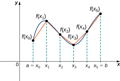
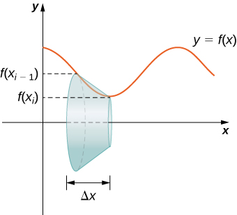
Let \( f(x)\) be a smooth function defined over \( [a,b]\). We want to calculate the length, \( L \), of the curve from the point \( (a,f(a))\) to the point \( (b,f(b))\). We start by using line segments to approximate the length of the curve. For \( i=0,1,2, \ldots ,n\), let \( P=\{x_i\}\) be a regular partition of \( [a,b]\). Then, for \( i=1,2, \ldots ,n\), construct a line segment from the point \( (x_{i−1},f(x_{i−1}))\) to the point \( (x_i,f(x_i))\). Although it might seem logical to use either horizontal or vertical line segments, we want our line segments to approximate the curve as closely as possible. Figure \(\PageIndex{1}\) depicts this construct for \( n=5\).
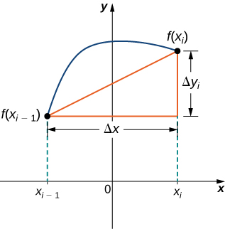
To help us find the length of each line segment, we look at the change in vertical distance as well as the change in horizontal distance over each interval. Because we have used a regular partition, the change in horizontal distance over each interval is given by \( \Delta x \). The change in vertical distance varies from interval to interval, though, so we use
\[ \Delta y_i =f(x_i) − f(x_{i−1}) \nonumber \]
to represent the change in vertical distance over the interval \( [x_{i−1},x_i]\), as shown in Figure \(\PageIndex{2}\).3 We will denote the length of the line segment from the point \( (x_{i−1},f(x_{i−1}))\) to the point \( (x_i,f(x_i))\) as \( l_i \).
By the Pythagorean Theorem, the length of the \( i^{\text{th}} \) line segment is
\[ \begin{array}{rcl}
l_i & = & \sqrt{( \Delta x)^2+( \Delta y_i)^2} \\
& = & \sqrt{1+\left( \frac{\Delta y_i}{\Delta x}\right)^2} \Delta x. \\
\end{array} \nonumber \]
Moreover, by the Mean Value Theorem, there is a point \( x^∗_i \in [x_{i−1},x_i]\) such that \( f^{\prime}(x^∗_i) = \frac{\Delta y_i}{\Delta x}\). Therefore, we can rewrite the last formula as
\[ l_i = \sqrt{1+[f^{\prime}(x^∗_i)]^2} \Delta x. \nonumber \]
Adding up the lengths of all the line segments, we get
\[L \equiv \text{Arc Length} \approx \sum_{i = 1}^n l_i = \sum_{i=1}^n\sqrt{1+[f^{\prime}(x^∗_i)]^2} \Delta x.\nonumber \]
This is a Riemann sum. Taking the limit as \( n \to \infty ,\) we have
\[\begin{array}{rcl}
L & = & \displaystyle \lim_{n \to \infty }\sum_{i=1}^n\sqrt{1+[f^{\prime}(x^∗_i)]^2} \Delta x \\
& = & \displaystyle \int^{x = b}_{x = a}\sqrt{1+[f^{\prime}(x)]^2} \, dx. \\
\end{array} \nonumber \]
Before we formalize all the work up to this point into a theorem, it is useful to create an arc length function, \( s(x) \), that allows us to find the length of the smooth curve \( f \) from the constant point \( \left( a,f(a) \right) \) to the arbitrary point \( \left( x,f(x) \right) \). Using our knowledge of integral functions, we determine that
\[ s(x) = \int_a^x \sqrt{1+[f^{\prime}(t)]^2} \, dt, \nonumber \]
is the arc length function.4 From the Fundamental Theorem of Calculus, Part 1 (FTC1) and our previous work with differentials,
\[ ds = s^{\prime}(x) dx \implies ds = \sqrt{1+[f^{\prime}(x)]^2} \, dx. \nonumber \]
We will discover throughout the remainder of this course that the differential we just found, \( ds \), has four equivalent forms. The choice of forms will depend on the structure of the curve with which we are working; however, in all forms the meaning of this differential is the same.
\( ds \) is the infinitesimal change in arc length given an infinitesimal change in some other value.
In our current case, \( ds \) is the infinitesimal change in arc length given an infinitesimal change in \( x \).
We now have enough mathematical language in place to streamline our discussion of arc length (and some other, future, topics). We summarize these findings in the following theorem.
Let \( f(x) \) be a smooth function over the interval \([a,b]\). Then the arc length, \( L \), of the portion of the graph of \( f(x) \) from the point \( (a,f(a)) \) to the point \( (b,f(b)) \) is given by
\[ L = \int_{x = a}^{x = b} \, ds, \label{ArcLengthWRTx} \]
where5
\[ds = \sqrt{1+[f^{\prime}(x)]^2}\,dx. \label{dsWRTx} \]
There are a few things that need to be pointed out about this previous theorem. First, the limits of the integral in Equation \( \ref{ArcLengthWRTx} \) are in terms of \( x \) - not \( s \). Therefore, evaluating Equation \( \ref{ArcLengthWRTx} \) as written is "mathematically illegal." Remember, to evaluate a definite integral, the limits of integration must be in terms of the variable of integration. Luckily, substituting in Equation \( \ref{dsWRTx} \) allows us to evaluate Equation \( \ref{ArcLengthWRTx} \) "legally."
This brings us to our next point. We did all that work to get \( ds \), but why not just say, "The arc length of \( f \) over \( [a,b] \) is
\[ L = \int_a^b \sqrt{1 + [f^{\prime}(x)]^2} \, dx\text{?"} \nonumber \]
As was mentioned prior to this theorem, \( ds \) will eventually have four equivalent (and often interchangeable) forms. Throughout these forms, the basic structure of the arc length integral, \( L = \int \, ds \), will not change - we will only need to worry about changing the limits of the integral and swapping out \( ds \) for an appropriate form.
Finally, note that we are integrating an expression involving \( f^{\prime}(x)\), so we need to be sure \( f^{\prime}(x)\) is integrable. This is why we require \( f(x)\) to be smooth.
The following example shows how to apply the theorem.
Let \( f(x)=2x^{3/2}\). Calculate the arc length of the graph of \( f(x)\) over the interval \( [0,1]\).
Solution
To get us into a "good habit," let's start by recognizing that \( f \) is a function of \( x \).6
We have \( f^{\prime}(x)=3x^{1/2},\) so \( [f^{\prime}(x)]^2=9x\). Therefore,
\[ ds = \sqrt{1+[f^{\prime}(x)]^2}\,dx = \sqrt{1+9x}\,dx. \nonumber \]
Then, the arc length is
\[ \begin{array}{rcll}
L & = & \displaystyle \int^{x = b}_{x = a} \, ds & \left( \text{The base arc length integral with limits in terms of }x \right) \\
& = & \displaystyle \int^{x = 1}_{x = 0}\sqrt{1+9x} \, dx & \\
& = & \dfrac{1}{9} \displaystyle \int^{u = 10}_{u = 1}\sqrt{u} \, du & \left( \text{Let }u = 1 + 9x \implies du = 9 \, dx\text{, and change the limits of integration accordingly} \right) \\
& = & \dfrac{1}{9} \cdot \dfrac{2}{3}u^{3/2}\bigg|^{10}_1 \\
& = & \dfrac{2}{27}[10\sqrt{10}−1] \\
\end{array} \nonumber \]
Let \(f(x)=(4/3)x^{3/2}\). Calculate the arc length of the graph of \( f(x)\) over the interval \( [0,1]\).
- Hint
-
Use the process from the previous example. Don’t forget to change the limits of integration.
- Answer
-
\[ \frac{1}{6}(5\sqrt{5}−1) \nonumber \]
Although it is nice to have a formula for calculating arc length, this particular theorem often generates expressions that are difficult to integrate. We will gain some ability to evaluate these integrals in the next chapter, but in some cases we may have to use a computer or calculator to approximate the value of the integral.
Let \( y = x^2\). Calculate the arc length of the graph of \( y \) over the interval \( [1,3]\).
Solution
Noting that \( y \) is a function of \( x \), we compute \( y^{\prime} = 2x,\) so that \( (y^{\prime})^2 = 4x^2\). Therefore,
\[ ds = \sqrt{1 + 4x^2} \, dx. \nonumber \]
Then the arc length is given by
\[ L = \int^{x = b}_{x = a} \, ds = \int^3_1\sqrt{1+4x^2}\,dx. \nonumber \]
Using the Right Endpoint Method with \( n = 10 \),7 we get
\[ \int ^3_1\sqrt{1+4x^2}\,dx \approx R_{10} = \sum_{n = 1}^{10} \sqrt{1 + 4 \left( 1 + \dfrac{1}{5}n \right)^2 } \cdot \dfrac{1}{5} \approx 8.65347. \nonumber \]
Let \( y = \sin(x)\). Calculate the arc length of the graph of \( y \) over the interval \( [0, \pi ]\). Use a computer or calculator to approximate the value of the integral.
- Hint
-
Use the process from the previous example.
- Answer
-
Depending on how many subintervals you choose (and whether you are using the Left Endpoint or the Right Endpoint Method), the value should approach
\[ \text{Arc Length} \approx 3.8202. \nonumber \]
2 This property comes up again in later chapters.
3 Note that some (or all) \( \Delta y_i\) may be negative.
4 To be clear, we defined the arc length of a given function over a constant interval using the dependent variable \( L \), but we defined the arc length function over a varying interval using the dependent variable \( s \).
5 There is often a confusion as to why we use \( s \) for the arc length function and \( L \) for the arc length of a curve. Why not just use \( s \) in both cases? In fact, wouldn't it make more sense to use \( s \) for the arc length of a curve given that we used \( s \) in Trigonometry for the arc length of the circle subtended by an angle \( \theta \)? The answer is more complex than most students care to hear, but since you are curious enough to investigate...
Recall that we arrived at the differential, \( ds \), by allowing \( s(x) = \displaystyle \int_a^x \sqrt{1+[f^{\prime}(t)]^2} \, dt\). This was all in an effort to streamline the eventual arc length formula into the simple statement in Equation \( \ref{ArcLengthWRTx} \). Had we also used the dependent variable \( s \) for this computed arc length, we would have arrived at
\[ s = \int_{x = a}^{x = b} \, ds. \nonumber \]
This would be completely nonsensical as we would be stating that the definite integral, which is a constant, is equal to \( s \); however, if \( s \) is constant, then its differential, \( ds \), would be 0, and so \( s \equiv 0 \) always.
6 I get it that this is obvious, but there is an actual reason for recognizing that this is a function of \( x \). We will see why in a little bit.
7 The choice of using the Right Endpoint Method as opposed to the Left Endpoint Method was completely arbitrary here, as was the decision to use \( n = 10 \) subintervals. In Differential Calculus, we were explicitly told what method to use and how many subintervals to consider, however, now that we are beyond that course, there will be times when we have to play the scientific investigator and make the decision of method and number of subintervals for ourselves.
Arc Length of the Curve \(x = g(y)\)
We have just seen how to approximate the length of a curve with line segments. If we want to find the arc length of the graph of a function of \(y\), we can repeat the same process, except we partition the \(y\)-axis instead of the \(x\)-axis. Figure \(\PageIndex{3}\) shows a representative line segment.
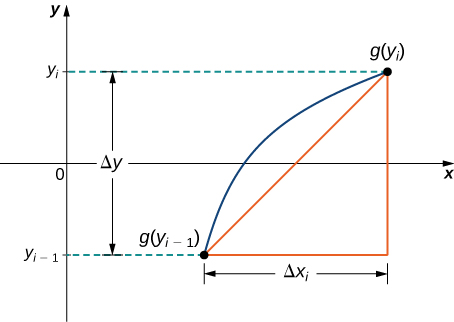
Then the length of the line segment is
\[l_i = \sqrt{( \Delta y)^2+( \Delta x_i)^2} = \sqrt{1+\left(\dfrac{ \Delta x_i}{ \Delta y}\right)^2} \Delta y. \nonumber \]
If we now follow the same development we did earlier, we get a formula for arc length of a function \(x=g(y)\).
Let \( g(y)\) be a smooth function over the (\( y \)-axis) interval \([c,d]\). Then the arc length, \( L \), of the portion of the graph of \( g(y)\) from the point \( (c,g(c))\) to the point \( (d,g(d))\) is given by
\[ L = \int_{y = c}^{y = d} \, ds, \nonumber \]
where8
\[ds = \sqrt{1+[g^{\prime}(y)]^2}\,dy. \label{dsWRTy} \]
Let \(x = 3y^3.\) Approximate the arc length of the curve over the (\( y \)-axis) interval \([1,2]\).
Solution
Note that \( x \) is definitely a function of \( y \). So we have \(x^{\prime} = 9y^2,\) so \((x^{\prime}(y))^2 = 81y^4\). Therefore,
\[ ds = \sqrt{1 + 81y^4} \, dy. \nonumber \]
Thus, the arc length is
\[ L = \int^{y = d}_{y = c} \, ds = \int^2_1\sqrt{1+81y^4}\,dy. \nonumber \]
\[ \begin{array}{rcl}
L & \approx & L_{20} \\
& = & \displaystyle \sum_{n = 1}^{20} \sqrt{1 + 81\left( 1 + \frac{1}{20}(n - 1) \right)^4} \cdot \dfrac{1}{20} \\
& \approx & 20.3576 \\
\end{array} \nonumber \]
Let \(g(y)=\frac{1}{y}\). Calculate the arc length of the graph of \(g(y)\) over the interval \([1,4]\). Use a computer or calculator to approximate the value of the integral.
- Hint
-
Use the process from the previous example.
- Answer
-
\[\text{Arc Length} \approx 3.15018 \nonumber \]
Arc Lengths - A Wealth of Choices
In the derivation of the arc length formulas, both with respect to \( x \) and with respect to \( y \), the base integral for arc length had the form
\[ s = \int \, ds, \nonumber \]
where \( s \) was the initial independent variable. We chose to trade out \( ds \) for an expression involving \( dx \) or \( dy \) depending on what we were learning at the moment; however, how would we know what form to use in a general scenario? Is the correct choice to trade out \( ds \) for an expression involving \( dx \)? Or would it be better to trade \( ds \) for its equivalent form in terms of \( dy \)? The good news is that there is a way to determine which option is viable. The bad news is that sometimes both options are viable and you have the extra work of determining which is the best to use.
Determining Which Form of \( ds \) to Use
Simply put, the form of \( ds \) available for use depends solely on whether the given curve is a function of \( x \), \( y \), or both over the given interval. That is, if the given curve is a function of \( x \) over the given interval, then
\[ ds = \sqrt{1 + [f^{\prime}(x)]^2} \, dx \nonumber \]
is a viable form. If the given curve is a function of \( y \) over the given interval, then
\[ ds = \sqrt{1 + [g^{\prime}(y)]^2} \, dy \nonumber \]
is a viable form. If the curve is both a function of \( x \) and a function of \( y \) over the given interval, then you can use either form of \( ds \); however, it is often the case that one such form will be easier to work with than the other.
Let's see this in an example.
Find the length of the curve \( y = \left( \frac{3}{2}x \right)^{2/3} + 1 \) on the (\( x \)-axis) interval \( \left[ 0, \frac{2}{3}(3)^{3/2} \right] \).
Solution
First, all arc length problems boil down to evaluating
\[ L = \int \, ds. \nonumber \]
We just need to determine the proper limits of integration and which form of \( ds \) to use. Since we were not explicitly told which variable to integrate with respect to, we need to do a little investigation.
With Respect to \( x \)
It's simple to see that, over the given interval of \( x \)-values, \( y \) is a function of \( x \). So we know that we can use \( ds = \sqrt{1 + [y^{\prime}(x)]^2} \, dx \). Let's setup the corresponding arc length integral to see how it looks.
\[ y^{\prime} = \dfrac{2}{3} \left( \dfrac{3}{2}x \right)^{-1/3} \cdot \dfrac{3}{2} = \left( \dfrac{3}{2}x \right)^{-1/3} \implies \left( y^{\prime} \right)^2 = \left( \dfrac{3}{2}x \right)^{-2/3}. \nonumber \]
Therefore, the arc length could be found by evaluating
\[ L = \int_{x = 0}^{x = \frac{2}{3}(3)^{3/2}} \sqrt{1 + \left( \dfrac{3}{2}x \right)^{-2/3}} \, dx. \nonumber \]
While not impossible to evaluate, the complex structure of this integrand should give you pause - especially when you know there might be way to approach this problem. Let's pause on this approach and see if the curve is a function of \( y \) over the given interval. If it's not, then we will come back to this and see if we can evaluate this integral analytically.10
With Respect to \( y \)
Solving the given equation for \( x \), we arrive at \( \left[\frac{2}{3} (y - 1)\right]^{3/2} = x \). This already looks uglier than the original equation, but do not let that stop you - Integral Calculus is full of pleasant surprises.
It should be somewhat obvious that \( x \) is a function of \( y \) wherever the function is defined (when \( y \geq 1 \)), so we should now investigate the interval of \( y \)-values corresponding to the original interval. When \( x = 0 \), \( y = 1 \), and when \( x = \frac{2}{3}(3)^{3/2} \), \( y = \left( \frac{3}{2} \cdot \frac{2}{3}(3)^{3/2} \right)^{2/3} + 1 = 3 + 1 = 4 \). Well... that's nice!
Finding the derivatives for the corresponding arc length integral, we get
\[ x^{\prime} = \dfrac{3}{2} \left[ \dfrac{2}{3}(y-1)\right]^{1/2} \cdot \dfrac{2}{3} = \left[ \dfrac{2}{3}(y-1)\right]^{1/2} \implies (x^{\prime})^2 = \dfrac{2}{3}(y-1). \nonumber \]
Hence, the arc length function is
\[ \begin{array}{rclr}
L & = & \displaystyle \int_{y = 1}^{y = 4} \sqrt{1 + \frac{2}{3}(y - 1)} \, dy & \\
& = & \displaystyle \int_{y = 1}^{y = 4} \sqrt{\frac{2}{3}y + \frac{1}{3}} \, dy & \\
& = & \dfrac{3}{2} \displaystyle \int_{u = 1}^{u = 3} \sqrt{u} \, du & \left( \text{Let }u=\frac{2}{3}y + \frac{1}{3} \implies du = \frac{2}{3} \, dy\text{, and change the limits of integration correspondingly} \right) \\
& = & \dfrac{3}{2} \cdot \dfrac{2}{3} u^{3/2}\bigg|_{u = 1}^{u = 3} & \\
& = & 3^{3/2} - 1 & \\
\end{array} \nonumber \]
Example \( \PageIndex{4} \) illustrates the need to investigate whether a given curve is a function of both \( x \) and \( y \) over a given interval. As we found, the difference in computational expense can be vastly different between approaches. I leave it to the reader to verify that the first integral (with respect to \( x \)) results in the same value as the second.11
Applications
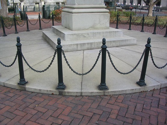
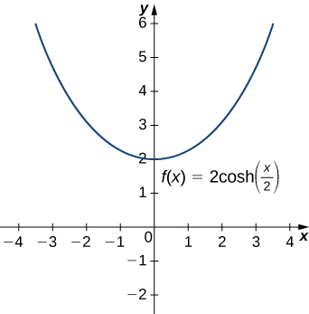
One physical application of hyperbolic functions involves hanging cables. If a cable of uniform density is suspended between two supports without any load other than its own weight, the cable forms a curve called a catenary. High-voltage power lines, chains hanging between two posts, and strands of a spider’s web all form catenaries. The following figure shows chains hanging from a row of posts.
Hyperbolic functions can be used to model catenaries. Specifically, functions of the form \(y = a \cdot \cosh\left(\frac{x}{a}\right)\) are catenaries. Figure \(\PageIndex{5}\) shows the graph of \(y=2\cosh\left(\frac{x}{2}\right)\).
Assume a hanging cable has the shape \(10\cosh\left(\frac{x}{10}\right)\) for \(−15 \leq x \leq 15\), where \(x\) is measured in feet. Determine the length of the cable (in feet).
Solution
We have \(f(x)=10 \cosh\left(\frac{x}{10}\right)\), so \(f^{\prime}(x) = \sinh\left(\frac{x}{10}\right)\). Then the arc length is
\[\int ^b_a\sqrt{1+[f^{\prime}(x)]^2} \, dx=\int ^{15}_{−15}\sqrt{1+\sinh^2 \left(\dfrac{x}{10}\right)} \, dx. \nonumber \]
Now recall that
\[1+\sinh^2x=\cosh^2x, \nonumber \]
so we have
\[\begin{array}{rcl}
\text{Arc Length} & = & \displaystyle \int ^{15}_{−15}\sqrt{1+\sinh^2 \left(\dfrac{x}{10}\right)} \, dx \\
& = & \displaystyle \int ^{15}_{−15}\cosh \left(\dfrac{x}{10}\right) \, dx \\
& = & 10\sinh \left(\dfrac{x}{10}\right)\bigg|^{15}_{−15} \\
& = & 10\left[\sinh\left(\dfrac{3}{2}\right)−\sinh\left(−\dfrac{3}{2}\right)\right] \\
& = & 20\sinh \left(\dfrac{3}{2}\right) \\
& \approx & 42.586\,\text{ft.} \\
\end{array} \nonumber \]
Assume a hanging cable has the shape \(15 \cosh\left(\frac{x}{15}\right)\) for \(−20 \leq x \leq 20\). Determine the length of the cable (in feet).
- Answer
-
\(52.95\) ft
Area of a Surface of Revolution
The concepts we used to find the arc length of a curve can be extended to find the surface area of a surface of revolution. Surface area is the total area of the outer layer of an object. For objects such as cubes or bricks, the surface area of the object is the sum of the areas of all of its faces. For curved surfaces, the situation is a little more complex. Let \(f(x)\) be a nonnegative smooth function over the interval \([a,b]\). We wish to find the surface area of the surface of revolution created by revolving the graph of \(y=f(x)\) around the \(x\)-axis as shown in the following figure.
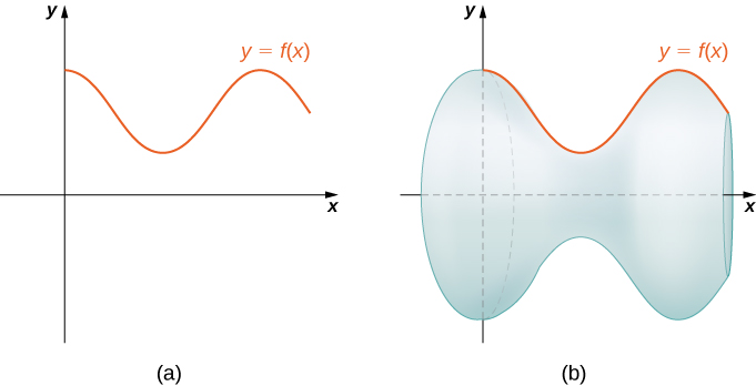
As we have done many times before, we are going to partition the interval \([a,b]\) and approximate the surface area by calculating the surface area of simpler shapes. We start by using line segments to approximate the curve, as we did earlier in this section. For \(i=0,1,2, \ldots ,n\), let \(P=\{x_i\}\) be a regular partition of \([a,b]\). Then, for \(i=1,2, \ldots ,n,\) construct a line segment from the point \((x_{i−1},f(x_{i−1}))\) to the point \((x_i,f(x_i))\). Now, revolve these line segments around the \(x\)-axis to generate an approximation of the surface of revolution as shown in the following figure.

Notice that when each line segment is revolved around the axis, it produces a band. These bands are actually pieces of cones.12 A piece of a cone like this is called a frustum of a cone.
12 Think of an ice cream cone with the pointy end cut off.
Deriving the Surface Area of a Frustum
In order to derive a formula for the surface area of the entire rotational volume, we must first focus our efforts on deriving a formula for the surface area of one of the bands of the overall rotated volume. To do so, we take a few steps back to Geometry.
To find the surface area of the band, we need to find the lateral surface area, \(S\), of the frustum.13 Let \(r_1\) and \(r_2\) be the radii of the wide end and the narrow end of the frustum, respectively, and let \(l\) be the slant height of the frustum as shown in the following figure.

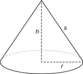
From Geometry, we know the lateral surface area of a cone is given by
\[\text{Lateral Surface Area} = \pi r s, \nonumber \]
where \(r\) is the radius of the base of the cone and \(s\) is the slant height (Figure \(\PageIndex{9}\)).
Since a frustum can be thought of as a piece of a cone, the lateral surface area of the frustum is given by the lateral surface area of the whole cone less the lateral surface area of the smaller cone (the pointy tip) that was cut off (Figure \(\PageIndex{10}\)).
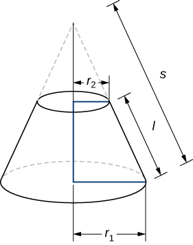
The cross-sections of the small cone and the large cone are similar triangles, so we see that
\[ \dfrac{r_2}{r_1} = \dfrac{s−l}{s}, \label{frustum1} \]
which can also be written as
\[ \dfrac{r_2 s}{r_1} = s−l. \label{frustum2} \]
Solving Equation \( \ref{frustum2} \) for \(s\), we get
\[ \begin{array}{rrcl}
& \dfrac{r_2 s}{r_1} & = & s−l \\
\implies & r_2s & = & r_1(s−l) \\
\implies & r_2s & = & r_1s−r_1 l \\
\implies & r_1l & = & r_1s−r_2s \\
\implies & r_1l & = & (r_1−r_2)s \\
\implies & \dfrac{r_1l}{r_1−r_2} & = & s \\
\end{array} \nonumber \]
We will use this last result,
\[ s = \dfrac{r_1l}{r_1−r_2}, \label{frustum3} \]
to help compute the surface area of the frustum.
If \( S \) is the surface area of the frustum, then
\[\begin{array}{rcll}
S & = & \text{(Lateral surface area of large cone)} - \text{(Lateral surface area of small cone)} & \\
& = & \pi r_1s - \pi r_2(s−l) & \\
& = & \pi r_1 s - \pi r_2(\dfrac{r_2 s}{r_1}) & \left( \text{from Equation }\ref{frustum2} \right) \\
& = & \pi s \left( r_1 - \dfrac{r_2^2}{r_1} \right) & \\
& = & \pi \left( \dfrac{r_1 l}{r_1 - r_2} \right) \left( \dfrac{r_1^2 - r_2^2}{r_1} \right) & \left( \text{from Equation }\ref{frustum3} \right) \\
& = & \pi \left( \dfrac{\cancel{r_1} l}{\cancel{(r_1 - r_2)}} \right) \left( \dfrac{\cancel{(r_1 - r_2)}(r_1 + r_2)}{\cancel{r_1}} \right) & \\
& = & \pi (r_1+r_2)l. \\
\nonumber \end{array} \]
Multiplying the numerator and denominator of this last result by 2, we get
\[ S = 2 \pi \left( \dfrac{r_1 + r_2}{2} \right) l = 2 \pi \bar{r} l, \label{frustum4} \]
where \( \bar{r} = \frac{r_1 + r_2}{2} \) is the average value of the radii of the band.
13 The area of just the slanted outside surface of the frustum, not including the areas of the top or bottom faces.
Deriving and Computing the Surface Area of a Rotational Volume
We now turn our attention back to the fact that we are rotating a function about an axis. To calculate the surface area of each of the bands formed by revolving the line segments around the \(x\)-axis, we consider the \( i^{\text{th}} \) subinterval and exchange \( l_i \) for \( l \). Moreover, without loss of generality, we can assume \( r_1 \) in our previous discussion is \( f(x_{i - 1}) \), and \( r_2 \) is \( f(x_i) \).14 The \( i^{\text{th}} \) band is shown in the following figure.
The surface area, \( S_i \), of this \( i^{\text{th}} \) band is therefore
\[\begin{array}{rcl}
S_i & = & 2 \pi \bar{r} l_i \\
& = & 2 \pi \left( \frac{f(x_{i−1}) + f(x_i)}{2} \right) \sqrt{1 + \left( f^{\prime}(x_i^*) \right)^2} \Delta x \\
\end{array} \nonumber \]
Furthermore, since \(f(x)\) is continuous, by the Intermediate Value Theorem, there is a point \(x^{**}_i \in [x_{i−1},x_i] \) such that \(f(x^{**}_i) = \frac{f(x_{i−1})+f(x_i)}{2} \), so we get
\[ S_i = 2 \pi f(x^{**}_i) \sqrt{1+(f^{\prime}(x^∗_i))^2} \Delta x.\nonumber \]
Then the approximate surface area of the whole surface of revolution is given by
\[S \equiv \text{Surface Area} \approx \sum_{i=1}^n 2 \pi f(x^{**}_i) \sqrt{1+(f^{\prime}(x^∗_i))^2} \Delta x.\nonumber \]
This almost looks like a Riemann sum, except we have functions evaluated at two different points, \(x^∗_i\) and \(x^{**}_{i}\), over the interval \([x_{i−1},x_i]\). Although we do not examine the details here, it turns out that because \(f(x)\) is smooth, if we let \(n \to \infty \), the limit works the same as a Riemann sum even with the two different evaluation points. This makes sense intuitively. Both \(x^∗_i\) and \(x^{**}_i\) are in the interval \([x_{i−1},x_i]\), so it makes sense that as \(n \to \infty \), both \(x^∗_i\) and \(x^{**}_i\) approach \(x\).15
Taking the limit as \(n \to \infty ,\) we get
\[ \begin{array}{rcl}
S \equiv \text{Surface Area} & = & \displaystyle \lim_{n \to \infty } \sum_{i=1}^n 2 \pi f(x^{**}_i) \sqrt{1+(f^{\prime}(x^∗_i))^2} \Delta x \\
& = & \displaystyle \int^{x = b}_{x = a} 2 \pi f(x) \sqrt{1+(f^{\prime}(x))^2})\, dx \\
\end{array} \nonumber \]
As with arc length, we can conduct a similar development for functions of \(y\) to get a formula for the surface area of surfaces of revolution about the \(y\)-axis. These findings are summarized in the following theorem.
The surface area of the surface of revolution formed by revolving the graph of a nonnegative, smooth function about an axis is
\[ S = \int_a^b 2 \pi r ds, \nonumber \]
where \( r \) is the radius of rotation and
\[ ds = \sqrt{1 + \left( f^{\prime}(x) \right)^2} dx \nonumber \]
or
\[ ds = \sqrt{1 + \left( g^{\prime}(y) \right)^2} dy. \nonumber \]
Recall, the differential \( ds \) represents an infinitesimal change in arc length. Which form you choose for \( ds \) will, again, depend on whether the given curve is a function of \( x \) or \( y \) (or both). The radius of rotation function, \( r \), is a function that gives the distance between the axis of rotation and the curve.
A great interpretation of the surface area integral
\[ \int 2 \pi r \, ds \nonumber \]
is that the surface area of the \( i^{\text{th}} \) band is the product of its circumference and its width. The circumference of the band is \( 2 \pi r_i \) and its width is \( \Delta s \).
Let \( f(x) = \sqrt{x}\) over the interval \([1,4]\). Find the surface area of the surface generated by revolving the graph of \(f(x)\) around the \(x\)-axis.
Solution
As always, begin by sketching the function, the volume, and a representative slice (not shown). The graph of \(f(x)\) and the surface of rotation are shown in Figure \(\PageIndex{12}\).
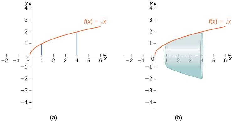
To showcase how flexible we can be, we are going to perform several different setups for this problem (we will only compute the value of one of them, as they all result in the same value).
With Respect to \( x \)
This is the approach most students would take because we know \( y = \sqrt{x} \) is a function of \( x \) on the given interval. Therefore, it makes sense to build an integral with respect to \( x \).
All surface area integrals have the common form
\[ S = \int 2 \pi r \, ds. \nonumber \]
Since we are rotating the curve about the \( x \)-axis, the radius of rotation is \( y_T - y_B = \sqrt{x} - 0 = \sqrt{x} \). Furthermore, replacing \( ds \) with a function of \( x \), we get
\[ \begin{array}{rcl}
ds & = & \sqrt{1 + (y^{\prime})^2} \, dx \\
& = & \sqrt{1 + \left(\frac{1}{2\sqrt{x}}\right)^2} \, dx \\
& = & \sqrt{1 + \frac{1}{4x}} \, dx
\end{array} \nonumber \]
Therefore,
\[\begin{array}{rclr}
S & = & \displaystyle \int^{x = b}_{x = a} 2 \pi r \, ds & \\
& = & \displaystyle \int^{x = 4}_{x = 1} 2 \pi \sqrt{x} \sqrt{1 + \frac{1}{4x}} \, dx & \\
& = & 2 \pi \displaystyle \int_{x = 1}^{x = 4} \sqrt{x} \sqrt{\frac{4x + 1}{4x}} \, dx & \\
& = & 2 \pi \displaystyle \int_{x = 1}^{x = 4} \frac{1}{2} \sqrt{4x + 1} \, dx & \\
& = & \pi \displaystyle \int_{x = 1}^{x = 4} \sqrt{4x + 1} \, dx & \\
& = & \frac{\pi}{4} \displaystyle \int_{u = 5}^{u = 17} \sqrt{u} \, du & \left( \text{Let }u=4x+1 \implies du = 4 \, dx\text{, and change the limits of integration accordingly} \right) \\
& = & \frac{\pi}{4} \cdot \frac{2}{3} u^{3/2} \bigg|_{u = 5}^{u = 17} & \\
& = & \frac{\pi}{6} \left(17^{3/2} - 5^{3/2}\right) & \\
\end{array} \nonumber \]
With Respect to \( y \)
This is not the approach most students would take, but I want to make certain that you understand all of your options. We were given \( y = \sqrt{x} \) on the \( x \)-interval \( \left[ 1,4 \right] \). On this interval, the curve is one-to-one. That is, it passes both the Vertical Line Test and the Horizontal Line Test. Hence, we could represent the curve as a function of \( y \) on this interval. Specifically, \( y^2 = x \) on the \( y \)-interval \( \left[ 1, 2 \right] \).
All surface area integrals have the common form
\[ S = \int 2 \pi r \, ds. \nonumber \]
Since we are rotating the curve about the \( x \)-axis, the radius of rotation is \( y_T - y_B = y - 0 = y \). Moreover, since we are choosing to integrate with respect to \( y \),
\[ ds = \sqrt{1 + (x^{\prime})^2} \, dy = \sqrt{1 + (2y)^2} \, dy = \sqrt{1 + 4y^2} \, dy. \nonumber \]
Putting this altogether, we get
\[ \begin{array}{rclr}
S & = & \displaystyle \int_{y=1}^{y =2} 2 \pi r \, ds & \\
& = & \displaystyle \int_{y = 1}^{y = 2} 2 \pi y \sqrt{1 + 4y^2} \, dy & \\
& = & 2 \pi \displaystyle \int_{y = 1}^{y = 2} y \sqrt{1 + 4y^2} \, dy & \\
& = & \frac{\pi}{4} \displaystyle \int_{u = 5}^{y = 17} \sqrt{u} \, du & \left( \text{Let }u = 1 + 4y^2 \implies du = 8y \, dy \text{, and change the limits of integration accordingly} \right) \\
& = & \frac{\pi}{4} \cdot \frac{2}{3} u^{3/2} \bigg|_{u = 5}^{u = 17} & \\
& = & \frac{\pi}{6} \left(17^{3/2} - 5^{3/2}\right) & \\
\end{array} \nonumber \]
Example \( \PageIndex{6} \) is another great illustration that knowing we have choice can simplify our computations. Integrating with respect to \( y \), while not the intuitive approach, led to a simpler integral.
Let \( f(x)=\sqrt{1−x}\) over the interval \( [0,1/2]\). Find the surface area of the surface generated by revolving the graph of \( f(x)\) around the \(x\)-axis.
- Hint
-
Use the process from the previous example.
- Answer
-
\[ \frac{ \pi }{6}(5\sqrt{5}−3\sqrt{3}) \nonumber \]
Let \( y= \sqrt[3]{3x}\). Consider the portion of the curve where \( 0 \leq y \leq 2\).
- Find the surface area of the surface generated by revolving the graph of \( f(x)\) around the \( y\)-axis.
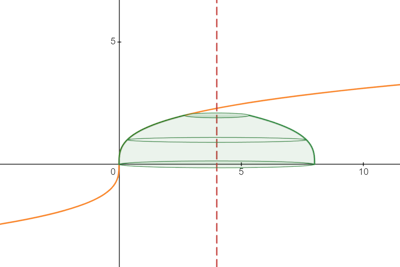
- Setup, but do not evaluate, and integral for the surface area of the surface generated by revolving the graph of \( f(x) \) about the line \( x = 4 \).
Solution
- A quick sketch of the curve, the solid, and a slice (not shown) is the starting point.
We know that all surface area integrals share the form\[ S = \int 2 \pi r \, ds. \nonumber \]If we decided to integrate with respect to \( x \), then the entire integrand must be written in terms of \( x \). The radius of rotation is \( x_R - x_L = x - 0 = x \) and our choice for \( ds \) would be\[ \begin{array}{rcl}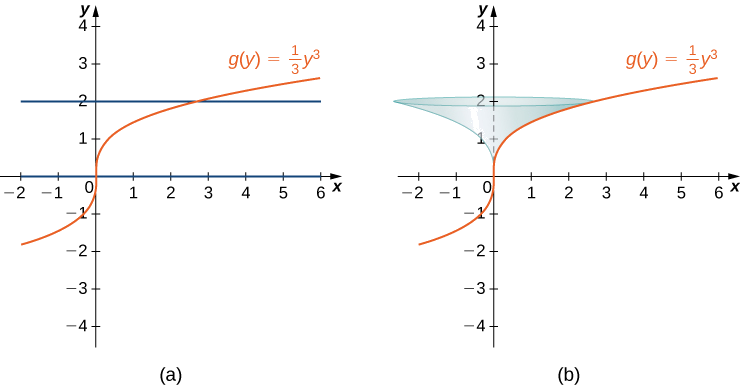
Figure \(\PageIndex{13}\): (a) The graph of \( g(y)\). (b) The surface of revolution.
ds & = & \sqrt{1 + (y^{\prime})^2} \, dx \\
& = & \sqrt{1 + \left( \frac{1}{3}(3x)^{-2/3} \cdot 3 \right)^2} \, dx \\
& = & \sqrt{1 + \left( (3x)^{-2/3} \right)^2} \, dx \\
& = & \sqrt{1 + (3x)^{-4/3}} \, dx \\ \end{array} \nonumber \]and so the surface area of this solid of revolution would be computed using\[ \begin{array}{rcl}
S & = & \displaystyle \int_{x = 0}^{x = 8/3} 2 \pi r \, ds \\
& = & 2 \pi \displaystyle \int_{x = 0}^{x = 8/3} x \sqrt{1 + (3x)^{-4/3}} \, dx \\
\end{array} \nonumber \]While we could evaluate this integral, it might be best to check if an integral in terms of \( y \) is cleaner.
Solving for \( x \), we have \( x = \frac{1}{3}y^3\), so \( x^{\prime} = y^2\) and \( (x^{\prime})^2 = y^4\). Moreover, the radius of rotation is \( x_R - x_L = \frac{1}{3}y^3 - 0 = \frac{1}{3}y^3 \). Hence,\[ \begin{array}{rclr}
S & = & \displaystyle \int_{y = 0}^{y = 2} 2 \pi r \, ds & \\
& = & 2 \pi \displaystyle \int_{y=0}^{y =2} \dfrac{1}{3}y^3 \sqrt{1 + y^4} \, dy & \\
& = & \dfrac{\pi}{6} \displaystyle \int_{u=1}^{u =17} \sqrt{u} \, du & \left( \text{Let }u = 1 + y^4 \implies du = 4y^3 \, dy\text{, and change the limits of integration accordingly} \right) \\
& = & \dfrac{\pi}{9} \cdot u^{3/2} \bigg|_{u=1}^{u =17} & \\
& = & \dfrac{\pi}{9} \left( 17^{3/2} - 1 \right) & \\
\end{array} \nonumber \] - A sketch of the curve and solid are shown below.
Building the integral with respect to \( y \) (I will leave building the integral with respect to \( x \) for the interested reader), we get\[ \begin{array}{rcl}
S & = & \displaystyle \int_{y = 0}^{y = 2} 2 \pi r \, ds \\
& = & 2 \pi \displaystyle \int_{y = 0}^{y = 2} \left( x_R - x_L \right) \, ds \\
& = & 2 \pi \displaystyle \int_{y = 0}^{y = 2} \left( 4 - \frac{1}{3} y^3 \right) \sqrt{1 + y^4} \, dy \\
\end{array} \nonumber \]Notice that the radius of rotation is the distance from the axis of rotation, \( x = 4 \), to the curve, \( x = \frac{1}{3} y^3 \). If you draw a radius line from the function to the axis of rotation, the right edge, \( x_R \), is at \( x = 4 \), and the left edge, \( x_L \), is at the curve, \( x = \frac{1}{3}y^3 \). This is why the value of \( r \) is \( 4 - \frac{1}{3}y^3 \).
Also note that \( ds \) didn't change. When rotating about a line that is not an axis, the only factor that changes in the formula for the surface area integral is \( r \) (because all you are doing is changing the radius of rotation).
Let \( g(y)=\sqrt{9−y^2}\) over the interval \( y \in [0,2]\). Find the surface area of the surface generated by revolving the graph of \( g(y)\) around the \( y\)-axis.
- Hint
-
Use the process from the previous example.
- Answer
-
\( 12 \pi \)
14 The phrase, "without loss of generality," is used quite extensively in mathematics. It means that, had the alternative situation occurred (in this case, had \( r_1 \) in our previous discussion been \( f(x_{i}) \) and \( r_2 \) been \( f(x_{i - 1}) \)), the results (with the appropriate adjustments) would be the same.
15 Those of you who are interested in the details should consult an advanced calculus text.
Key Concepts
- The arc length of a curve can be calculated using a definite integral.
- The arc length is first approximated using line segments, which generates a Riemann sum. Taking a limit then gives us the definite integral formula. The same process can be applied to functions of \( y\).
- The concepts used to calculate the arc length can be generalized to find the surface area of a surface of revolution.
- The integrals generated by both the arc length and surface area formulas are often difficult to evaluate. It may be necessary to use a computer or calculator to approximate the values of the integrals.
Key Equations
- Arc Length of a Function of x
Arc Length \( = \int ^b_a\sqrt{1+[f^{\prime}(x)]^2}dx\)
- Arc Length of a Function of y
Arc Length \( = \int ^d_c\sqrt{1+[g′(y)]^2}dy\)
- Surface Area of a Function of x
Surface Area \( = \int ^b_a(2 \pi f(x)\sqrt{1+(f^{\prime}(x))^2})dx\)
Glossary
- arc length
- the arc length of a curve can be thought of as the distance a person would travel along the path of the curve
- frustum
- a portion of a cone; a frustum is constructed by cutting the cone with a plane parallel to the base
- surface area
- the surface area of a solid is the total area of the outer layer of the object; for objects such as cubes or bricks, the surface area of the object is the sum of the areas of all of its faces