Mathematics LibreTexts

1.2: Determining Volumes by Slicing

  • Page ID
    163249
  • \( \newcommand{\vecs}[1]{\overset { \scriptstyle \rightharpoonup} {\mathbf{#1}} } \)

    \( \newcommand{\vecd}[1]{\overset{-\!-\!\rightharpoonup}{\vphantom{a}\smash {#1}}} \)

    \( \newcommand{\id}{\mathrm{id}}\) \( \newcommand{\Span}{\mathrm{span}}\)

    ( \newcommand{\kernel}{\mathrm{null}\,}\) \( \newcommand{\range}{\mathrm{range}\,}\)

    \( \newcommand{\RealPart}{\mathrm{Re}}\) \( \newcommand{\ImaginaryPart}{\mathrm{Im}}\)

    \( \newcommand{\Argument}{\mathrm{Arg}}\) \( \newcommand{\norm}[1]{\| #1 \|}\)

    \( \newcommand{\inner}[2]{\langle #1, #2 \rangle}\)

    \( \newcommand{\Span}{\mathrm{span}}\)

    \( \newcommand{\id}{\mathrm{id}}\)

    \( \newcommand{\Span}{\mathrm{span}}\)

    \( \newcommand{\kernel}{\mathrm{null}\,}\)

    \( \newcommand{\range}{\mathrm{range}\,}\)

    \( \newcommand{\RealPart}{\mathrm{Re}}\)

    \( \newcommand{\ImaginaryPart}{\mathrm{Im}}\)

    \( \newcommand{\Argument}{\mathrm{Arg}}\)

    \( \newcommand{\norm}[1]{\| #1 \|}\)

    \( \newcommand{\inner}[2]{\langle #1, #2 \rangle}\)

    \( \newcommand{\Span}{\mathrm{span}}\) \( \newcommand{\AA}{\unicode[.8,0]{x212B}}\)

    \( \newcommand{\vectorA}[1]{\vec{#1}}      % arrow\)

    \( \newcommand{\vectorAt}[1]{\vec{\text{#1}}}      % arrow\)

    \( \newcommand{\vectorB}[1]{\overset { \scriptstyle \rightharpoonup} {\mathbf{#1}} } \)

    \( \newcommand{\vectorC}[1]{\textbf{#1}} \)

    \( \newcommand{\vectorD}[1]{\overrightarrow{#1}} \)

    \( \newcommand{\vectorDt}[1]{\overrightarrow{\text{#1}}} \)

    \( \newcommand{\vectE}[1]{\overset{-\!-\!\rightharpoonup}{\vphantom{a}\smash{\mathbf {#1}}}} \)

    \( \newcommand{\vecs}[1]{\overset { \scriptstyle \rightharpoonup} {\mathbf{#1}} } \)

    \( \newcommand{\vecd}[1]{\overset{-\!-\!\rightharpoonup}{\vphantom{a}\smash {#1}}} \)

    \(\newcommand{\avec}{\mathbf a}\) \(\newcommand{\bvec}{\mathbf b}\) \(\newcommand{\cvec}{\mathbf c}\) \(\newcommand{\dvec}{\mathbf d}\) \(\newcommand{\dtil}{\widetilde{\mathbf d}}\) \(\newcommand{\evec}{\mathbf e}\) \(\newcommand{\fvec}{\mathbf f}\) \(\newcommand{\nvec}{\mathbf n}\) \(\newcommand{\pvec}{\mathbf p}\) \(\newcommand{\qvec}{\mathbf q}\) \(\newcommand{\svec}{\mathbf s}\) \(\newcommand{\tvec}{\mathbf t}\) \(\newcommand{\uvec}{\mathbf u}\) \(\newcommand{\vvec}{\mathbf v}\) \(\newcommand{\wvec}{\mathbf w}\) \(\newcommand{\xvec}{\mathbf x}\) \(\newcommand{\yvec}{\mathbf y}\) \(\newcommand{\zvec}{\mathbf z}\) \(\newcommand{\rvec}{\mathbf r}\) \(\newcommand{\mvec}{\mathbf m}\) \(\newcommand{\zerovec}{\mathbf 0}\) \(\newcommand{\onevec}{\mathbf 1}\) \(\newcommand{\real}{\mathbb R}\) \(\newcommand{\twovec}[2]{\left[\begin{array}{r}#1 \\ #2 \end{array}\right]}\) \(\newcommand{\ctwovec}[2]{\left[\begin{array}{c}#1 \\ #2 \end{array}\right]}\) \(\newcommand{\threevec}[3]{\left[\begin{array}{r}#1 \\ #2 \\ #3 \end{array}\right]}\) \(\newcommand{\cthreevec}[3]{\left[\begin{array}{c}#1 \\ #2 \\ #3 \end{array}\right]}\) \(\newcommand{\fourvec}[4]{\left[\begin{array}{r}#1 \\ #2 \\ #3 \\ #4 \end{array}\right]}\) \(\newcommand{\cfourvec}[4]{\left[\begin{array}{c}#1 \\ #2 \\ #3 \\ #4 \end{array}\right]}\) \(\newcommand{\fivevec}[5]{\left[\begin{array}{r}#1 \\ #2 \\ #3 \\ #4 \\ #5 \\ \end{array}\right]}\) \(\newcommand{\cfivevec}[5]{\left[\begin{array}{c}#1 \\ #2 \\ #3 \\ #4 \\ #5 \\ \end{array}\right]}\) \(\newcommand{\mattwo}[4]{\left[\begin{array}{rr}#1 \amp #2 \\ #3 \amp #4 \\ \end{array}\right]}\) \(\newcommand{\laspan}[1]{\text{Span}\{#1\}}\) \(\newcommand{\bcal}{\cal B}\) \(\newcommand{\ccal}{\cal C}\) \(\newcommand{\scal}{\cal S}\) \(\newcommand{\wcal}{\cal W}\) \(\newcommand{\ecal}{\cal E}\) \(\newcommand{\coords}[2]{\left\{#1\right\}_{#2}}\) \(\newcommand{\gray}[1]{\color{gray}{#1}}\) \(\newcommand{\lgray}[1]{\color{lightgray}{#1}}\) \(\newcommand{\rank}{\operatorname{rank}}\) \(\newcommand{\row}{\text{Row}}\) \(\newcommand{\col}{\text{Col}}\) \(\renewcommand{\row}{\text{Row}}\) \(\newcommand{\nul}{\text{Nul}}\) \(\newcommand{\var}{\text{Var}}\) \(\newcommand{\corr}{\text{corr}}\) \(\newcommand{\len}[1]{\left|#1\right|}\) \(\newcommand{\bbar}{\overline{\bvec}}\) \(\newcommand{\bhat}{\widehat{\bvec}}\) \(\newcommand{\bperp}{\bvec^\perp}\) \(\newcommand{\xhat}{\widehat{\xvec}}\) \(\newcommand{\vhat}{\widehat{\vvec}}\) \(\newcommand{\uhat}{\widehat{\uvec}}\) \(\newcommand{\what}{\widehat{\wvec}}\) \(\newcommand{\Sighat}{\widehat{\Sigma}}\) \(\newcommand{\lt}{<}\) \(\newcommand{\gt}{>}\) \(\newcommand{\amp}{&}\) \(\definecolor{fillinmathshade}{gray}{0.9}\)

    Volume and the Slicing Method

    Let’s motivate a new theorem (the basis for all future theorems on volumes).

    Theorem: Volume of a Solid - The Slicing Method

    The volume of a solid is\[ V = \displaystyle \lim_{n \to \infty} \sum_{i = 1}^n A\left( \lambda_i^* \right) \Delta \lambda = \int_a^b A(\lambda) \, d \lambda, \nonumber \]where \(A(\lambda_i^* )\) is the cross-sectional area at the \(i^{th}\) slice and \( \Delta \lambda \) is the "thickness" of the slice.

    Non-Rotational Volumes

    Common Volumes

    Lecture Example \(\PageIndex{1}\)

    Find the volume of a pyramid with height \(h\) and rectangular base with dimensions \(b\) and \(2b\).

    Uncommon Volumes

    Interactive Element: Volumes of Known Cross-Sections
     

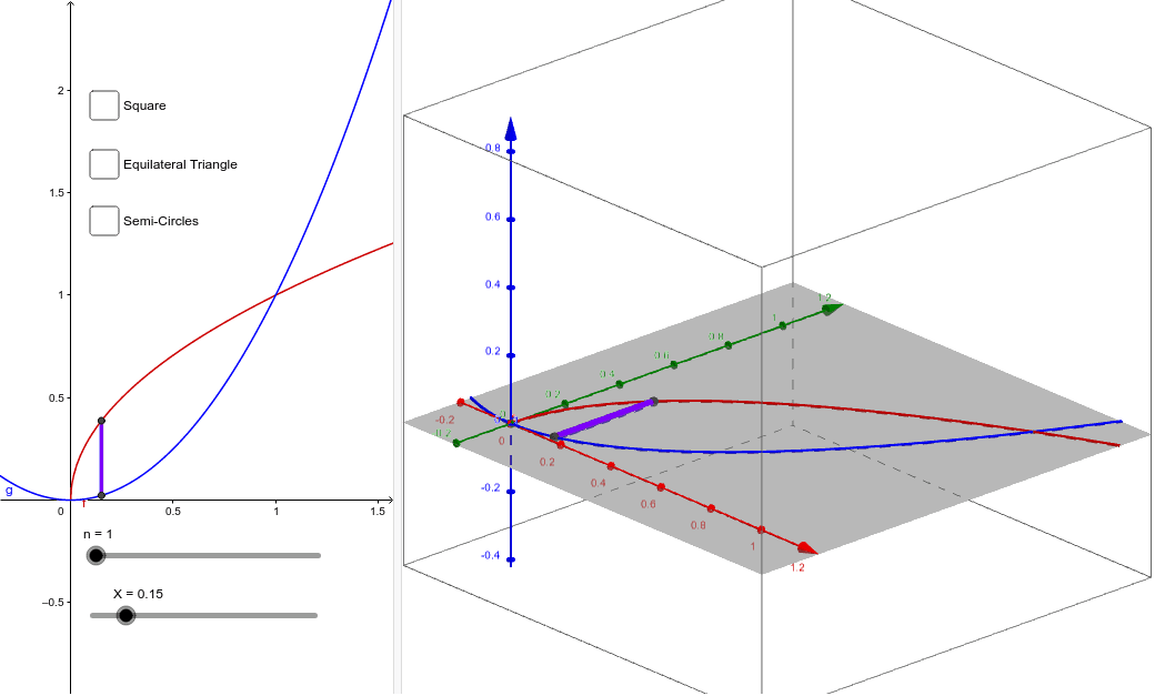
    Description: This Geogebra applet allows you to visualize how a solid of known cross-sections is generated by placing cross-sectional slices perpendicular to the \( x \)-axis on a base defined by the boundary between two function (red and blue) from \( x = 0 \) to \( X \), where you can adjust \( X \) using the bottom slider.

    Interact: Adjust the rightmost boundary, \( X \), of the region to whatever value you want, select a single cross-sectional shape (square, equilateral triangle, or semi-circle), increase \( n \) to a decent number of slices to help you visualize what is going on, and (finally) use your mouse to adjust the graph of the right side of the applet to see the resulting solid.

    Interactive Element: Solids of Known Cross-Sections

    Solids of Known Cross Section | Wolfram Demonstrations Project

    Lecture Example \(\PageIndex{2}\)

    Find the volume of the solid with the base being the elliptical region \(9x^2+4y^2=36\), where cross-sections perpendicular to the \(x\)-axis are isosceles right triangles with hypotenuse in the base.

    Rotational Volumes

    The Disk Method

    Interactive Element: Volumes Using the Disk Method

    Volumes Using the Disc Method | Wolfram Demonstrations Project

    Theorem: The Volume of a Rotational Solid - The Disk Method

    Let \(f(\lambda)\) be continuous on an interval \( \lambda = a \) to \( \lambda = b \). The volume obtained by rotating this function about the \( \lambda \)-axis is\[ V = \displaystyle  \int_{\lambda=a}^{\lambda = b} A\left( \lambda \right) \, d\lambda, \nonumber \]where \( A\left( \lambda \right) = \pi r\left( \lambda \right)^2 \) is the cross-sectional area at \( \lambda \). Hence,\[ V = \displaystyle \int_{\lambda=a}^{\lambda = b} \pi r\left( \lambda \right)^2 \, d\lambda. \nonumber \]

    Lecture Example \(\PageIndex{3}\)

    Find the volume of the solid obtained by rotating the region bounded by\[y=e^x, \quad y=0, \quad x=-1, \quad x=1\nonumber \]about the \(x\)-axis.

    The Washer Method

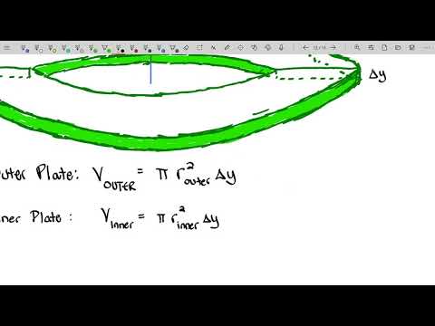
    What if someone wanted to drill a hole in our rotational solid?

    Interactive Element: Drilled-Out Volumes

    Solid of Revolution | Wolfram Demonstrations Project

    Theorem: The Washer Method

    If the region to be rotated is bounded by the functions \(f\left( \lambda \right)\) and \(g\left( \lambda \right)\), then\[A\left( \lambda \right)= \pi \left[ \left( \text{outer radius} \right)^2 - \left( \text{inner radius} \right)^2 \right]. \nonumber \]

    Caution

    A very common mistake is to think that the volume in the previous theorem is\[\int ^b_a \pi \left[f(x)−g(x)\right]^2\,dx \nonumber \](if rotating about the \( x \)-axis). This is why I strongly encourage not to memorize that formula, but instead to derive it until it makes sense. I will demonstrate this process with each remaining problem.

    Lecture Example \(\PageIndex{4}\)

    Find the volume of the solid obtained by rotating the region bounded by\[ y^2 = x, \quad x = 2y \nonumber \]about the \(y\)-axis.

    Lecture Example \(\PageIndex{5}\)
    Vote for One of the Following!

    Find the volume of the solid obtained by rotating the region bounded by\[y=1+\sec⁡(x), \quad y=3\nonumber \]about \(y=1\).

    - OR -

    Determine the volume of the solid obtained by rotating the region bounded by \[y=\cos⁡(x), \quad y=\sin⁡(x)\nonumber \]about \(y=-1\) on the interval \( \left[ 0,\frac{\pi}{4} \right] \).

    Synthesis Questions

    Online Lecture Example \(\PageIndex{6}\)

    Set up an integral for the volume of a solid torus with radii \(r\) and \(R\). By interpreting the integral as an area, find the volume of the torus.


    This page titled 1.2: Determining Volumes by Slicing is shared under a CC BY-NC-SA 4.0 license and was authored, remixed, and/or curated by Roy Simpson.