2.2: Basics of the Graphing Calculator


- Last updated
- Sep 12, 2022
- Save as PDF

( \newcommand{\kernel}{\mathrm{null}\,}\)
It’s time to learn how to use a graphing calculator to sketch the graph of an equation. We will use the TI-84 silver edition graphing calculator in this section, but the skills we introduce will work equally well similar older TI-83 graphing calculators as well as other TI-84 models. Screen views may be slightly different between the different calculator models but the features are all the same.

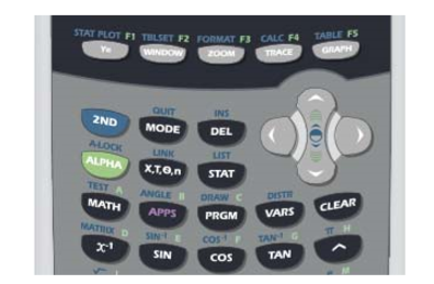
In this introduction to the graphing calculator, you will need to use several keys on the upper half of the graphing calculator (see Figure 2.2.2). The up-and-down and left-and-right arrow keys are located in the upper right corner of Figure 2.2.2. These are used for moving the cursor on the calculator view screen and various menus. Immediately below these arrow keys is the CLEAR button, used to clear the view screen and equations in the Y= menu.
It is not uncommon that people share their graphing calculators with friends who make changes to the settings in the calculator. Let’s take a moment to make sure we have some common settings on our calculators.
Above each button are one or more commands located on the calculator’s case. Press the 2ND key to access a command having the same color as the 2ND key. Press the ALPHA key to access a command having the same color as the ALPHA key.
Locate and push the MODE in the first row of Figure 2.2.2. This will open the window shown in Figure 2.2.3. Make sure that the mode settings on your calculator are identical to the ones shown in Figure 2.2.3. If not, use the up-and-down arrow keys to move to the non-matching line item. This should place a blinking cursor over the first item on the line. Press the ENTER button on the lower-right corner of your calculator to make the selection permanent. Once you’ve completed your changes, press 2ND MODE again to quit the MODE menu.
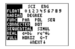
The QUIT command is located above the MODE button on the calculator case and is used to exit the current menu.
Next, note the buttons across the first row of the calculator, located immediately below the view screen.

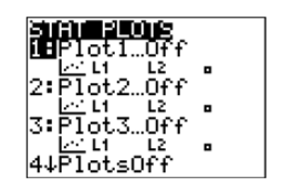
We need all of the stat plots to be “off.” If any of the three stat plots are “on,” select 4:PlotsOff (press the number 4 on your keyboard), then press the ENTER key on the lower right corner of your calculator. That’s it! Your calculator should now be ready for the upcoming You Trys.
Use the graphing calculator to sketch the graph of y=x+1.
Solution
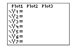
Press the Y= button. The window shown in Figure 2.2.5 appears. If any equations appear in the Y= menu of Figure 2.2.5, use the up-and-down arrow keys and the CLEAR button (located below the up-and-down and left-and-right arrow keys) to delete them.
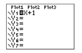
Next, move the cursor to Y1=, then enter the equation y=x+1 in Y1 with the following button keystrokes. The result is shown in Figure 2.2.6.

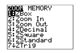
There are two ways to make this selection:
- Use the down-arrow key to move downward in the ZOOM menu until 6:ZStandard is highlighted, then press the ENTER key.
- A quicker alternative is to simply press the number 6 on the calculator keyboard to select 6:ZStandard.
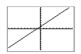
The resulting graph of y=x+1 is shown in Figure 2.2.8.
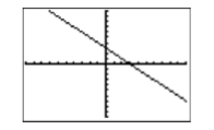
Use the graphing calculator to sketch the graph of y=−x+3.
- Answer
-
Use the graphing calculator to sketch the graph of y=x2−7.
Solution
Press the Y= button and enter the equation y=x2−7 into Y1 (see Figure 2.2.9) with the following keystrokes:

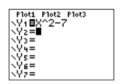
The caret (∧) symbol (see Figure 2.2.2) is located in the last column of buttons on the calculator, just underneath the CLEAR button, and means “raised to.” The caret button is used for entering exponents. For example, x2 is entered as X∧2, x3 is entered as X∧3, and so on.
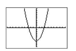
Press the ZOOM button, then select 6:ZStandard from the ZOOM menu to produce the graph of y=x2−7 shown in Figure 2.2.10.
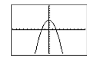
Use the graphing calculator to sketch the graph of y=−x2+4.
- Answer
-
Standard Window Parameters and Adjusting the Viewing Window
Consider again the final result of Example 2.2.2 shown in Figure 2.2.10. To determine the scale at each end of each axis, press the WINDOW button on the topmost row of buttons on your calculator. The WINDOW settings for Figure 2.2.10 are shown below in Figure 2.2.11. Figure 2.2.12 presents a visual explanation of each of the entries Xmin,Xmax,Ymin and Ymax.
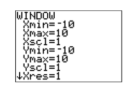
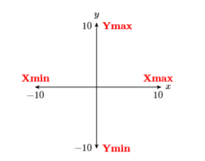
Xmin and Xmax indicate the scale at the left- and right-hand ends of the x-axis, respectively, while Ymin and Ymax indicate the scale at the bottomand top-ends of the y-axis. Finally, as we shall see shortly, Xscl and Yscl control the spacing between tick marks on the x- and y-axes, respectively.
Note that Figure 2.2.12 gives us some sense of the meaning of the “standard viewing window” produced by selecting 6:ZStandard from the ZOOM menu. Each time you select 6:ZStandard from the ZOOM menu, Xmin is set to −10, Xmax to 10, and Xscl to 1 (distance between the tick marks on the x-axis). Similarly, Ymin is set to −10, Ymax to 10, and Yscl to 1 (distance between the tick marks on the y-axis). You can, however, override these settings as we shall see in the next example.
Sketch the graphs of the following equations on the same viewing screen.
y=54x−3 and y=23x+4
Adjust the viewing window so that the point at which the graphs intersect (where the graphs cross one another) is visible in the viewing window, then use the TRACE button to approximate the coordinates of the point of intersection.
Solution
We must first decide on the proper syntax to use when entering the equations. In the case of the first equation, note that
y=54x−3
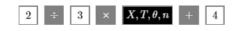
is pronounced “y equals five-fourths x minus three,” and means “y equals five-fourths times x minus three.” Enter this equation into Y1 in the Y= menu as 5/4∗X−3 (see Figure 2.2.13), using the button keystrokes:
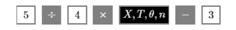
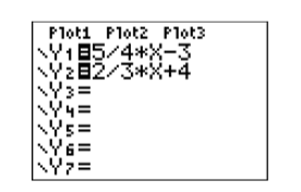
The division and times buttons are located in the rightmost column of the calculator. Similarly, enter the second equation into Y2 as 2/3∗X+4 using the button keystrokes:
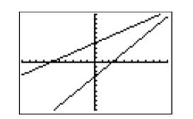
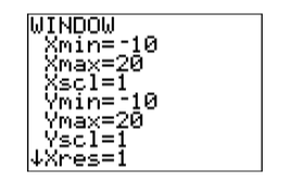
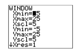
When we examine the resulting graphs in Figure 2.2.15, it appears that their point of intersection will occur off the screen above and to the right of the upper right-corner of the current viewing window. With this thought in mind, let’s extend the x-axis to the right by increasing the value of Xmax to 20. Further, let’s extend the y-axis upward by increasing the value of Ymin to 20. Press the WINDOW button on the top row of the calculator, then make the adjustments shown in Figure 2.2.16.
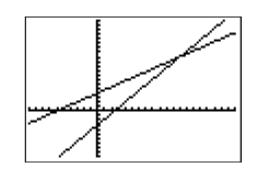
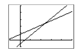
If we select 6:ZStandard from the ZOOM menu, our changes to the WINDOW parameters will be discarded and the viewing window will be returned to the “standard viewing window.” If we want to keep our changes to the WINDOW parameters, the correct approach at this point is to push the GRAPH button on the top row of the calculator. The resulting graph is shown in Figure 2.2.17. Note that the point of intersection of the two lines is now visible in the viewing window.
The image in Figure 2.2.17 is ready for recording onto your homework. However, we think we would have a better picture if we made a couple more changes:
- It would be nicer if the point of intersection were more centered in the viewing window.
- There are far too many tick marks.
With these thoughts in mind, make the changes to the WINDOW parameters shown in Figure 2.2.18, then push the GRAPH button to produce the image in Figure 2.2.19.
Finally, push the TRACE button on the top row of buttons, then use the left- and right-arrow keys to move the cursor atop the point of intersection. An approximation of the coordinates of the point of intersection are reported at the bottom of the viewing window (see Figure 2.2.20).
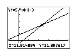
The TRACE button is only capable of providing a very rough approximation of the point of intersection. In Chapter 4, we’ll introduce the intersection utility on the CALC menu, which will report a much more accurate result.
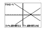
Approximate the point of intersection of the graphs of y=x−4 and y=5−x using the TRACE button.
- Answer
-
(4.68,0.68)