
2.4: Adding and Subtracting Polynomial Expressions
- Page ID
- 92359

\( \newcommand{\vecs}[1]{\overset { \scriptstyle \rightharpoonup} {\mathbf{#1}} } \)
\( \newcommand{\vecd}[1]{\overset{-\!-\!\rightharpoonup}{\vphantom{a}\smash {#1}}} \)
\( \newcommand{\dsum}{\displaystyle\sum\limits} \)
\( \newcommand{\dint}{\displaystyle\int\limits} \)
\( \newcommand{\dlim}{\displaystyle\lim\limits} \)
\( \newcommand{\id}{\mathrm{id}}\) \( \newcommand{\Span}{\mathrm{span}}\)
( \newcommand{\kernel}{\mathrm{null}\,}\) \( \newcommand{\range}{\mathrm{range}\,}\)
\( \newcommand{\RealPart}{\mathrm{Re}}\) \( \newcommand{\ImaginaryPart}{\mathrm{Im}}\)
\( \newcommand{\Argument}{\mathrm{Arg}}\) \( \newcommand{\norm}[1]{\| #1 \|}\)
\( \newcommand{\inner}[2]{\langle #1, #2 \rangle}\)
\( \newcommand{\Span}{\mathrm{span}}\)
\( \newcommand{\id}{\mathrm{id}}\)
\( \newcommand{\Span}{\mathrm{span}}\)
\( \newcommand{\kernel}{\mathrm{null}\,}\)
\( \newcommand{\range}{\mathrm{range}\,}\)
\( \newcommand{\RealPart}{\mathrm{Re}}\)
\( \newcommand{\ImaginaryPart}{\mathrm{Im}}\)
\( \newcommand{\Argument}{\mathrm{Arg}}\)
\( \newcommand{\norm}[1]{\| #1 \|}\)
\( \newcommand{\inner}[2]{\langle #1, #2 \rangle}\)
\( \newcommand{\Span}{\mathrm{span}}\) \( \newcommand{\AA}{\unicode[.8,0]{x212B}}\)
\( \newcommand{\vectorA}[1]{\vec{#1}} % arrow\)
\( \newcommand{\vectorAt}[1]{\vec{\text{#1}}} % arrow\)
\( \newcommand{\vectorB}[1]{\overset { \scriptstyle \rightharpoonup} {\mathbf{#1}} } \)
\( \newcommand{\vectorC}[1]{\textbf{#1}} \)
\( \newcommand{\vectorD}[1]{\overrightarrow{#1}} \)
\( \newcommand{\vectorDt}[1]{\overrightarrow{\text{#1}}} \)
\( \newcommand{\vectE}[1]{\overset{-\!-\!\rightharpoonup}{\vphantom{a}\smash{\mathbf {#1}}}} \)
\( \newcommand{\vecs}[1]{\overset { \scriptstyle \rightharpoonup} {\mathbf{#1}} } \)
\(\newcommand{\longvect}{\overrightarrow}\)
\( \newcommand{\vecd}[1]{\overset{-\!-\!\rightharpoonup}{\vphantom{a}\smash {#1}}} \)
\(\newcommand{\avec}{\mathbf a}\) \(\newcommand{\bvec}{\mathbf b}\) \(\newcommand{\cvec}{\mathbf c}\) \(\newcommand{\dvec}{\mathbf d}\) \(\newcommand{\dtil}{\widetilde{\mathbf d}}\) \(\newcommand{\evec}{\mathbf e}\) \(\newcommand{\fvec}{\mathbf f}\) \(\newcommand{\nvec}{\mathbf n}\) \(\newcommand{\pvec}{\mathbf p}\) \(\newcommand{\qvec}{\mathbf q}\) \(\newcommand{\svec}{\mathbf s}\) \(\newcommand{\tvec}{\mathbf t}\) \(\newcommand{\uvec}{\mathbf u}\) \(\newcommand{\vvec}{\mathbf v}\) \(\newcommand{\wvec}{\mathbf w}\) \(\newcommand{\xvec}{\mathbf x}\) \(\newcommand{\yvec}{\mathbf y}\) \(\newcommand{\zvec}{\mathbf z}\) \(\newcommand{\rvec}{\mathbf r}\) \(\newcommand{\mvec}{\mathbf m}\) \(\newcommand{\zerovec}{\mathbf 0}\) \(\newcommand{\onevec}{\mathbf 1}\) \(\newcommand{\real}{\mathbb R}\) \(\newcommand{\twovec}[2]{\left[\begin{array}{r}#1 \\ #2 \end{array}\right]}\) \(\newcommand{\ctwovec}[2]{\left[\begin{array}{c}#1 \\ #2 \end{array}\right]}\) \(\newcommand{\threevec}[3]{\left[\begin{array}{r}#1 \\ #2 \\ #3 \end{array}\right]}\) \(\newcommand{\cthreevec}[3]{\left[\begin{array}{c}#1 \\ #2 \\ #3 \end{array}\right]}\) \(\newcommand{\fourvec}[4]{\left[\begin{array}{r}#1 \\ #2 \\ #3 \\ #4 \end{array}\right]}\) \(\newcommand{\cfourvec}[4]{\left[\begin{array}{c}#1 \\ #2 \\ #3 \\ #4 \end{array}\right]}\) \(\newcommand{\fivevec}[5]{\left[\begin{array}{r}#1 \\ #2 \\ #3 \\ #4 \\ #5 \\ \end{array}\right]}\) \(\newcommand{\cfivevec}[5]{\left[\begin{array}{c}#1 \\ #2 \\ #3 \\ #4 \\ #5 \\ \end{array}\right]}\) \(\newcommand{\mattwo}[4]{\left[\begin{array}{rr}#1 \amp #2 \\ #3 \amp #4 \\ \end{array}\right]}\) \(\newcommand{\laspan}[1]{\text{Span}\{#1\}}\) \(\newcommand{\bcal}{\cal B}\) \(\newcommand{\ccal}{\cal C}\) \(\newcommand{\scal}{\cal S}\) \(\newcommand{\wcal}{\cal W}\) \(\newcommand{\ecal}{\cal E}\) \(\newcommand{\coords}[2]{\left\{#1\right\}_{#2}}\) \(\newcommand{\gray}[1]{\color{gray}{#1}}\) \(\newcommand{\lgray}[1]{\color{lightgray}{#1}}\) \(\newcommand{\rank}{\operatorname{rank}}\) \(\newcommand{\row}{\text{Row}}\) \(\newcommand{\col}{\text{Col}}\) \(\renewcommand{\row}{\text{Row}}\) \(\newcommand{\nul}{\text{Nul}}\) \(\newcommand{\var}{\text{Var}}\) \(\newcommand{\corr}{\text{corr}}\) \(\newcommand{\len}[1]{\left|#1\right|}\) \(\newcommand{\bbar}{\overline{\bvec}}\) \(\newcommand{\bhat}{\widehat{\bvec}}\) \(\newcommand{\bperp}{\bvec^\perp}\) \(\newcommand{\xhat}{\widehat{\xvec}}\) \(\newcommand{\vhat}{\widehat{\vvec}}\) \(\newcommand{\uhat}{\widehat{\uvec}}\) \(\newcommand{\what}{\widehat{\wvec}}\) \(\newcommand{\Sighat}{\widehat{\Sigma}}\) \(\newcommand{\lt}{<}\) \(\newcommand{\gt}{>}\) \(\newcommand{\amp}{&}\) \(\definecolor{fillinmathshade}{gray}{0.9}\)In this section we concentrate on adding and subtracting polynomial expressions, based on earlier work combining like terms in Ascending and Descending Powers. Let’s begin with an addition example.
Simplify: \[\left(a^{2}+3 a b-b^{2}\right)+\left(4 a^{2}+11 a b-9 b^{2}\right) \nonumber \]
Solution
Use the commutative and associative properties to change the order and regroup. Then combine like terms.
\[\begin{aligned}\left(a^{2}+3 a b-b^{2}\right) &+\left(4 a^{2}+11 a b-9 b^{2}\right) \\ &=\left(a^{2}+4 a^{2}\right)+(3 a b+11 a b)+\left(-b^{2}-9 b^{2}\right) \\ &=5 a^{2}+14 a b-10 b^{2} \end{aligned} \nonumber \]
Simplify: \(\left(3 s^{2}-2 s t+4 t^{2}\right)+\left(s^{2}+7 t s-5 t^{2}\right)\)
- Answer
-
\(4 s^{2}+5 s t-t^{2}\)
If you are comfortable skipping a step or two, it is not necessary to write down all of the steps shown in Example \(\PageIndex{1}\). Let’s try combining like terms mentally in the next example.
Simplify: \[\left(x^{3}-2 x^{2} y+3 x y^{2}+y^{3}\right)+\left(2 x^{3}-4 x^{2} y-8 x y^{2}+5 y^{3}\right) \nonumber \]
Solution
If we use the associative and commutative property to reorder and regroup, then combine like terms, we get the following result.
\[\begin{aligned}\left(x^{3}-2 x^{2} y\right.&+3 x y^{2}+y^{3} )+\left(2 x^{3}-4 x^{2} y-8 x y^{2}+5 y^{3}\right) \\ &=\left(x^{3}+2 x^{3}\right)+\left(-2 x^{2} y-4 x^{2} y\right)+\left(3 x y^{2}-8 x y^{2}\right)+\left(y^{3}+5 y^{3}\right) \\ &=3 x^{3}-6 x^{2} y-5 x y^{2}+6 y^{3} \end{aligned} \nonumber \]
However, if we can combine like terms mentally, eliminating the middle step, it is much more efficient to write:
\[\begin{array}{l}{\left(x^{3}-2 x^{2} y+3 x y^{2}+y^{3}\right)+\left(2 x^{3}-4 x^{2} y-8 x y^{2}+5 y^{3}\right)} \\ {\quad \quad=3 x^{3}-6 x^{2} y-5 x y^{2}+6 y^{3}}\end{array} \nonumber \]
Simplify: \(\left(-5 a^{2} b+4 a b-3 a b^{2}\right)+\left(2 a^{2} b+7 a b-a b^{2}\right)\)
- Answer
-
\(-3 a^{2} b+11 a b-4 a b^{2}\)
Negating a Polynomial
Before attempting subtraction of polynomials, let’s first address how to negate or “take the opposite” of a polynomial. First recall that negating is equivalent to multiplying by \(−1\).
If \(a\) is any number, then
\[−a =(−1)a. \nonumber \]
That is, negating is equivalent to multiplying by \(−1\).
We can use this property to simplify \(−(a + b)\). First, negating is identical to multiplying by \(−1\). Then we can distribute the \(−1\).
\[\begin{aligned} -(a+b) &= (-1)(a+b) \qquad \color {Red} \text { Negating is equivalent to multiplying by } -1 \\ &= (-1) a+(-1) b \qquad \color {Red} \text { Distribute the }-1 . \\ &= -a+(-b) \qquad \color {Red} \text { Simplify: }(-1) a=-a \text { and }(-1) b=-b \\ &= -a-b \qquad \color {Red} \text { Subtraction means add the opposite. } \end{aligned} \nonumber \]
Thus, \(−(a + b)=−a −b\). However, it is probably simpler to note that the minus sign in front of the parentheses simply changed the sign of each term inside the parentheses.
When negating a sum of terms, the effect of the minus sign is to change each term in the parentheses to the opposite sign. \[−(a + b)=−a−b\nonumber\]
Let’s look at this principle in the next example.
Simplify: \(-\left(-3 x^{2}+4 x-8\right)\)
Solution
First, negating is equivalent to multiplying by \(−1\). Then distribute the \(−1\).
\[\begin{aligned} -&\left(-3 x^{2}+4 x-8\right) \\ &=(-1)\left(-3 x^{2}+4 x-8\right) \qquad \color {Red} \text{Negating is equivalent to multiplying by } -1\\ &=(-1)\left(-3 x^{2}\right)+(-1)(4 x)-(-1)(8) \qquad \color {Red} \text {Distribute the } -1 \\ &=3 x^{2}+(-4 x)-(-8) \qquad \color {Red} \text {Simplify: } (-1)(-3 x^{2})=3 x^{2}, (-1)(4 x)=-4 x, \text {and} (-1)(8)=-8\\ &=3 x^{2}-4 x+8 \qquad \color {Red} \text {Subtraction means add the opposite.} \end{aligned} \nonumber \]
Alternate solution:
As we saw above, a negative sign in front of a parentheses simply changes the sign of each term inside the parentheses. So it is much more efficient to write\[−(−3x^2 +4x−8) = 3x^2 −4x +8 \nonumber \]simply changing the sign of each term inside the parentheses.
Simplify: \(-\left(2 x^{2}-3 x+9\right)\)
- Answer
-
\(-2 x^{2}+3 x-9\)
Subtracting Polynomials
Now that we know how to negate a polynomial (change the sign of each term of the polynomial), we’re ready to subtract polynomials.
Simplify: \(\left(y^{3}-3 y^{2} z+4 y z^{2}+z^{3}\right)-\left(2 y^{3}-8 y^{2} z+2 y z^{2}-8 z^{3}\right)\)
Solution
First, distribute the minus sign, changing the sign of each term of the second polynomial.
\[\left(y^{3}-3 y^{2} z+4 y z^{2}+z^{3}\right)-\left(2 y^{3}-8 y^{2} z+2 y z^{2}-8 z^{3}\right)=y^{3}-3 y^{2} z+4 y z^{2}+z^{3}-2 y^{3}+8 y^{2} z-2 y z^{2}+8 z^{3} \nonumber \]
Regroup, combining like terms. You may perform this next step mentally if you wish.
\[\begin{array}{l}{=\left(y^{3}-2 y^{3}\right)+\left(-3 y^{2} z+8 y^{2} z\right)+\left(4 y z^{2}-2 y z^{2}\right)+\left(z^{3}+8 z^{3}\right)} \\ {=-y^{3}+5 y^{2} z+2 y z^{2}+9 z^{3}}\end{array} \nonumber \]
Simplify: \(\left(4 a^{2} b+2 a b-7 a b^{2}\right)-\left(2 a^{2} b-a b-5 a b^{2}\right)\)
- Answer
-
\(2 a^{2} b+3 a b-2 a b^{2}\)
Some Applications
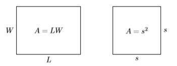
Recall that the area of a rectangle having length \(L\) and width \(W\) is found using the formula \(A = LW\). The area of a square having side s is found using the formula \(A = s^2\) (see Figure \(\PageIndex{1}\)).
Find the area of the square in Figure \(\PageIndex{2}\) by summing the area of its parts.
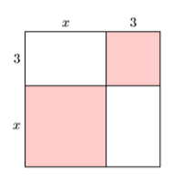
Solution
Let’s separate each of the four pieces and label each with its area (see Figure \(\PageIndex{3}\)).
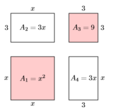
The two shaded squares in Figure \(\PageIndex{3}\) have areas \(A_1 = x^2\) and \(A_3 = 9\), respectively. The two unshaded rectangles in Figure \(\PageIndex{3}\) have areas \(A_2 =3 x\) and \(A_4 =3x\). Summing these four areas gives us the area of the entire figure.
\[\begin{aligned} A &=A_{1}+A_{2}+A_{3}+A_{4} \\ &=x^{2}+3 x+9+3 x \\ &=x^{2}+6 x+9 \end{aligned} \nonumber \]
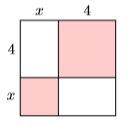
Find the area of the square shown below by summing the area of its parts.
- Answer
-
\(x^{2}+8 x+16\)