
10.2: Calculus with Parametric Curves


- Last updated
- Jan 23, 2021
- Save as PDF
( \newcommand{\kernel}{\mathrm{null}\,}\)
- Determine derivatives and equations of tangents for parametric curves.
- Find the area under a parametric curve.
- Use the equation for arc length of a parametric curve.
- Apply the formula for surface area to a volume generated by a parametric curve.
Now that we have introduced the concept of a parameterized curve, our next step is to learn how to work with this concept in the context of calculus. For example, if we know a parameterization of a given curve, is it possible to calculate the slope of a tangent line to the curve? How about the arc length of the curve? Or the area under the curve?
Another scenario: Suppose we would like to represent the location of a baseball after the ball leaves a pitcher’s hand. If the position of the baseball is represented by the plane curve (x(t),y(t)) then we should be able to use calculus to find the speed of the ball at any given time. Furthermore, we should be able to calculate just how far that ball has traveled as a function of time.
Derivatives of Parametric Equations
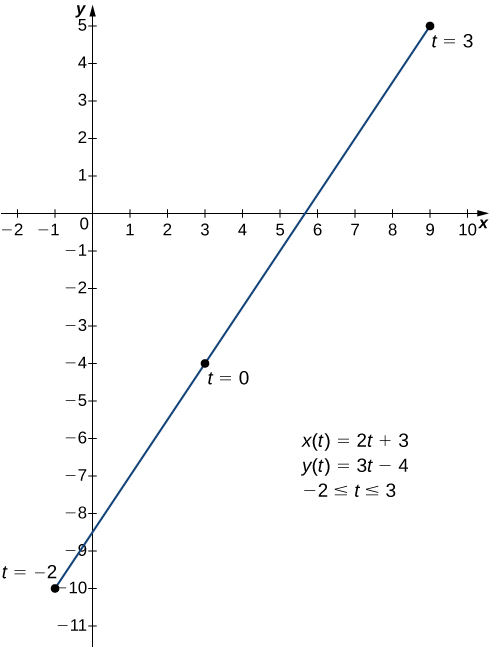
We start by asking how to calculate the slope of a line tangent to a parametric curve at a point. Consider the plane curve defined by the parametric equations
x(t)=2t+3y(t)=3t−4
within −2≤t≤3.
The graph of this curve appears in Figure 10.2.1. It is a line segment starting at (−1,−10) and ending at (9,5).
We can eliminate the parameter by first solving Equation 10.2.1 for t:
x(t)=2t+3
x−3=2t
t=x−32.
Substituting this into y(t) (Equation 10.2.2), we obtain
y(t)=3t−4
y=3(x−32)−4
y=3x2−92−4
y=3x2−172.
The slope of this line is given by dydx=32. Next we calculate x′(t) and y′(t). This gives x′(t)=2 and y′(t)=3. Notice that
dydx=dy/dtdx/dt=32.
This is no coincidence, as outlined in the following theorem.
Consider the plane curve defined by the parametric equations x=x(t) and y=y(t). Suppose that x′(t) and y′(t) exist, and assume that x′(t)≠0. Then the derivative dydx is given by
dydx=dy/dtdx/dt=y′(t)x′(t).
This theorem can be proven using the Chain Rule. In particular, assume that the parameter t can be eliminated, yielding a differentiable function y=F(x). Then y(t)=F(x(t)). Differentiating both sides of this equation using the Chain Rule yields
y′(t)=F′(x(t))x′(t),
so
F′(x(t))=y′(t)x′(t).
But F′(x(t))=dydx, which proves the theorem.
□
Equation ??? can be used to calculate derivatives of plane curves, as well as critical points. Recall that a critical point of a differentiable function y=f(x) is any point x=x0 such that either f′(x0)=0 or f′(x0) does not exist. Equation ??? gives a formula for the slope of a tangent line to a curve defined parametrically regardless of whether the curve can be described by a function y=f(x) or not.
Calculate the derivative dydx for each of the following parametrically defined plane curves, and locate any critical points on their respective graphs.
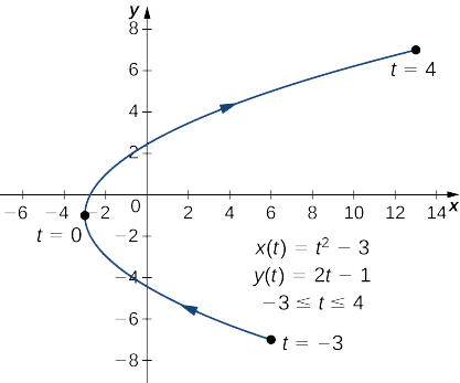
- x(t)=t2−3,y(t)=2t−1,for −3≤t≤4
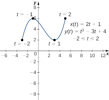
- x(t)=2t+1,y(t)=t3−3t+4,for −2≤t≤2
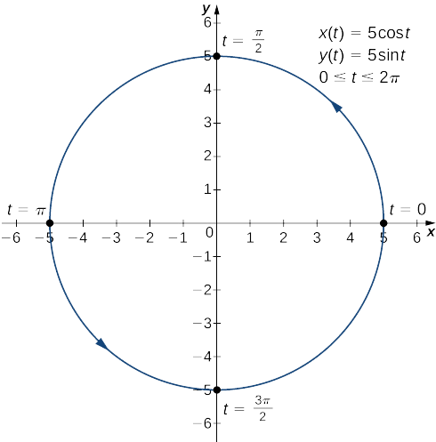
- x(t)=5cost,y(t)=5sint,for 0≤t≤2π
Solution
a. To apply Equation ???, first calculate x′(t) and y′(t):
x′(t)=2t
y′(t)=2.
Next substitute these into the equation:
dydx=dy/dtdx/dt
dydx=22t
dydx=1t.
This derivative is undefined when t=0. Calculating x(0) and y(0) gives x(0)=(0)2−3=−3 and y(0)=2(0)−1=−1, which corresponds to the point (−3,−1) on the graph. The graph of this curve is a parabola opening to the right, and the point (−3,−1) is its vertex as shown.
b. To apply Equation ???, first calculate x′(t) and y′(t):
x′(t)=2
y′(t)=3t2−3.
Next substitute these into the equation:
dydx=dy/dtdx/dt
dydx=3t2−32.
This derivative is zero when t=±1. When t=−1 we have
x(−1)=2(−1)+1=−1 and y(−1)=(−1)3−3(−1)+4=−1+3+4=6,
which corresponds to the point (−1,6) on the graph. When t=1 we have
x(1)=2(1)+1=3 and y(1)=(1)3−3(1)+4=1−3+4=2,
which corresponds to the point (3,2) on the graph. The point (3,2) is a relative minimum and the point (−1,6) is a relative maximum, as seen in the following graph.
c. To apply Equation ???, first calculate x′(t) and y′(t):
x′(t)=−5sint
y′(t)=5cost.
Next substitute these into the equation:
dydx=dy/dtdx/dt
dydx=5cost−5sint
dydx=−cott.
This derivative is zero when cost=0 and is undefined when sint=0. This gives t=0,π2,π,3π2, and 2π as critical points for t. Substituting each of these into x(t) and y(t), we obtain
| t | x(t) | y(t) |
|---|---|---|
| 0 | 5 | 0 |
| π2 | 0 | 5 |
| π | −5 | 0 |
| 3π2 | 0 | −5 |
| 2π | 5 | 0 |
These points correspond to the sides, top, and bottom of the circle that is represented by the parametric equations (Figure 10.2.4). On the left and right edges of the circle, the derivative is undefined, and on the top and bottom, the derivative equals zero.
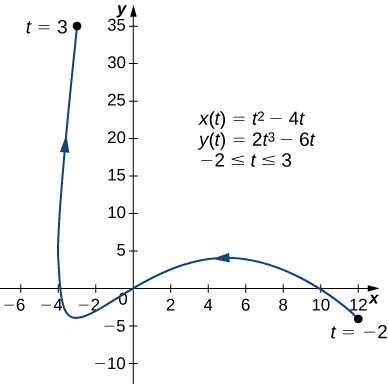
Calculate the derivative dy/dx for the plane curve defined by the equations
x(t)=t2−4t,y(t)=2t3−6t,for −2≤t≤3
and locate any critical points on its graph.
- Hint
-
Calculate x′(t) and y′(t) and use Equation ???.
- Answer
-
x′(t)=2t−4 and y′(t)=6t2−6, so dydx=6t2−62t−4=3t2−3t−2.
This expression is undefined when t=2 and equal to zero when t=±1.
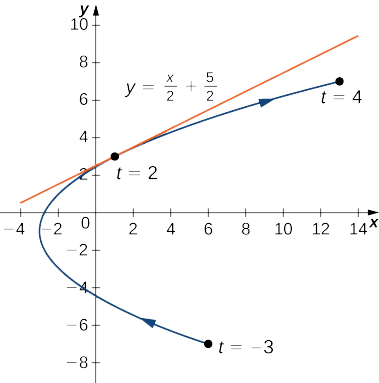
Find the equation of the tangent line to the curve defined by the equations
x(t)=t2−3,y(t)=2t−1,for −3≤t≤4
when t=2.
Solution
First find the slope of the tangent line using Equation ???, which means calculating x′(t) and y′(t):
x′(t)=2t
y′(t)=2.
Next substitute these into the equation:
dydx=dy/dtdx/dt
dydx=22t
dydx=1t.
When t=2,dydx=12, so this is the slope of the tangent line. Calculating x(2) and y(2) gives
x(2)=(2)2−3=1 and y(2)=2(2)−1=3,
which corresponds to the point (1,3) on the graph (Figure 10.2.5). Now use the point-slope form of the equation of a line to find the equation of the tangent line:
y−y0=m(x−x0)
y−3=12(x−1)
y−3=12x−12
y=12x+52.
Find the equation of the tangent line to the curve defined by the equations
x(t)=t2−4t,y(t)=2t3−6t,for −2≤t≤6 when t=5.
- Hint
-
Calculate x′(t) and y′(t) and use Equation ???.
- Answer
-
The equation of the tangent line is y=24x+100.
Second-Order Derivatives
Our next goal is to see how to take the second derivative of a function defined parametrically. The second derivative of a function y=f(x) is defined to be the derivative of the first derivative; that is,
d2ydx2=ddx[dydx].
Since
dydx=dy/dtdx/dt,
we can replace the y on both sides of Equation ??? with dydx. This gives us
d2ydx2=ddx(dydx)=(d/dt)(dy/dx)dx/dt.
If we know dy/dx as a function of t, then this formula is straightforward to apply
Calculate the second derivative d2y/dx2 for the plane curve defined by the parametric equations x(t)=t2−3,y(t)=2t−1,for −3≤t≤4.
Solution
From Example 10.2.1 we know that dydx=22t=1t. Using Equation ???, we obtain
d2ydx2=(d/dt)(dy/dx)dx/dt=(d/dt)(1/t)2t=−t−22t=−12t3.
Calculate the second derivative d2y/dx2 for the plane curve defined by the equations
x(t)=t2−4t,y(t)=2t3−6t,for −2≤t≤3
and locate any critical points on its graph.
- Hint
-
Start with the solution from the previous exercise, and use Equation ???.
- Answer
-
d2ydx2=3t2−12t+32(t−2)3. Critical points (5,4),(−3,−4),and (−4,6).
Integrals Involving Parametric Equations
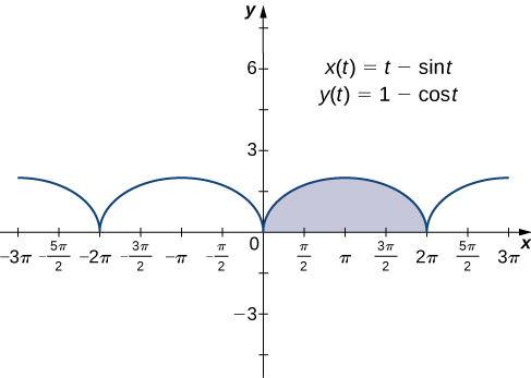
Now that we have seen how to calculate the derivative of a plane curve, the next question is this: How do we find the area under a curve defined parametrically? Recall the cycloid defined by these parametric equations
x(t)=t−sinty(t)=1−cost.
Suppose we want to find the area of the shaded region in the following graph.
To derive a formula for the area under the curve defined by the functions
x=x(t)y=y(t)
where a≤t≤b.
We assume that x(t) is differentiable and start with an equal partition of the interval a≤t≤b. Suppose t0=a<t1<t2<⋯<tn=b and consider the following graph.
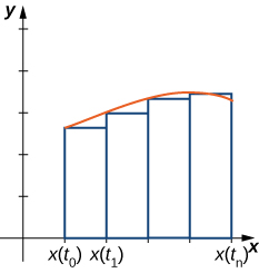
We use rectangles to approximate the area under the curve. The height of a typical rectangle in this parametrization is y(x(¯ti)) for some value ¯ti in the ith subinterval, and the width can be calculated as x(ti)−x(ti−1). Thus the area of the ith rectangle is given by
Ai=y(x(¯ti))(x(ti)−x(ti−1)).
Then a Riemann sum for the area is
An=n∑i=1y(x(¯ti))(x(ti)−x(ti−1)).
Multiplying and dividing each area by ti−ti−1 gives
An=n∑i=1y(x(¯ti))(x(ti)−x(ti−1)ti−ti−1)(ti−ti−1)=n∑i=1y(x(¯ti))(x(ti)−x(ti−1)Δt)Δt.
Taking the limit as n approaches infinity gives
A=lim
This leads to the following theorem.
Consider the non-self-intersecting plane curve defined by the parametric equations
x=x(t),\quad y=y(t),\quad \text{for }a≤t≤b \nonumber
and assume that x(t) is differentiable. The area under this curve is given by
A=\int^b_ay(t)x′(t)\,dt.\label{ParaArea}
Find the area under the curve of the cycloid defined by the equations
x(t)=t−\sin t, \quad y(t)=1−\cos t, \quad \text{for }0≤t≤2π. \nonumber
Solution
Using Equation \ref{ParaArea}, we have
\begin{align*} A &=\int^b_ay(t)x′(t)\,dt\\[4pt] &=\int^{2π}_0(1−\cos t)(1−\cos t)\,dt\\[4pt] &=\int^{2π}_0(1−2\cos t+\cos^2t)\,dt\\[4pt] &=\int^{2π}_0\left(1−2\cos t+\dfrac{1+\cos (2t)}{2}\right)\,dt\\[4pt] &=\int^{2π}_0\left(\dfrac{3}{2}−2\cos t+\dfrac{\cos (2t)}{2}\right)\,dt\\[4pt] &=\dfrac{3t}{2}−2\sin t+\dfrac{\sin (2t)}{4}∣^{2π}_0\\[4pt] &=3π\end{align*}
Find the area under the curve of the hypocycloid defined by the equations
x(t)=3\cos t+\cos(3t), \quad y(t)=3\sin t−\sin(3t), \quad \text{for }0≤t≤π. \nonumber
- Hint
-
Use Equation \ref{ParaArea}, along with the identities \sin α\sin β=\dfrac{1}{2}[\cos(α−β)−\cos(α+β)] and \sin^2t=\dfrac{1−\cos (2t)}{2}.
- Answer
-
A=3π (Note that the integral formula actually yields a negative answer. This is due to the fact that x(t) is a decreasing function over the interval [0,π]; that is, the curve is traced from right to left.)
Arc Length of a Parametric Curve
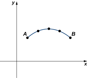
In addition to finding the area under a parametric curve, we sometimes need to find the arc length of a parametric curve. In the case of a line segment, arc length is the same as the distance between the endpoints. If a particle travels from point A to point B along a curve, then the distance that particle travels is the arc length. To develop a formula for arc length, we start with an approximation by line segments as shown in the following graph.
Given a plane curve defined by the functions x=x(t),\quad y=y(t),\quad \text{for }a≤t≤b, we start by partitioning the interval [a,b] into n equal subintervals: t_0=a<t_1<t_2<⋯<t_n=b. The width of each subinterval is given by Δt=(b−a)/n. We can calculate the length of each line segment:
d_1=\sqrt{(x(t_1)−x(t_0))^2+(y(t_1)−y(t_0))^2} \nonumber
d_2=\sqrt{(x(t_2)−x(t_1))^2+(y(t_2)−y(t_1))^2} \nonumber
etc.
Then add these up. We let s denote the exact arc length and s_n denote the approximation by n line segments:
s≈\sum_{k=1}^ns_k=\sum_{k=1}^n\sqrt{(x(t_k)−x(t_{k−1}))^2+(y(t_k)−y(t_{k−1}))^2}. \label{arc5}
If we assume that x(t) and y(t) are differentiable functions of t, then the Mean Value Theorem applies, so in each subinterval [t_{k−1},t_k] there exist \hat{t_k} and \tilde{t_k} such that
x(t_k)−x(t_{k−1})=x′(\hat{t_k})(t_k−t_{k−1})=x′(\hat{t_k})\,Δt \nonumber
y(t_k)−y(t_{k−1})=y′(\tilde{t_k})(t_k−t_{k−1})=y′(\tilde{t_k})\,Δt. \nonumber
Therefore Equation \ref{arc5} becomes
\begin {align*} s ≈\sum_{k=1}^ns_k &=\sum_{k=1}^n\sqrt{(x′(\hat{t_k})Δt)^2+(y′(\tilde{t_k})Δt)^2} \\[4pt] &=\sum_{k=1}^n\sqrt{(x′(\hat{t_k}))^2(Δt)^2+(y′(\tilde{t_k}))^2(Δt)^2} \\[4pt] &=\sum_{k=1}^n\sqrt{(x′(\hat{t_k}))^2+(y′(\tilde{t_k}))^2}Δt. \end{align*}
This is a Riemann sum that approximates the arc length over a partition of the interval [a,b]. If we further assume that the derivatives are continuous and let the number of points in the partition increase without bound, the approximation approaches the exact arc length. This gives
\begin{align*} s &=\lim_{n→∞}\sum_{k=1}^ns_k \\[4pt] &=\lim_{n→∞}\sum_{k=1}^n\sqrt{(x′(\hat{t_k}))^2+(y′(\tilde{t_k}))^2}Δt \\[4pt] &=\int^b_a\sqrt{(x′(t))^2+(y′(t))^2}\,dt . \end{align*}
When taking the limit, the values of \hat{t_k} and \tilde{t_k} are both contained within the same ever-shrinking interval of width Δt, so they must converge to the same value.
We can summarize this method in the following theorem.
Consider the plane curve defined by the parametric equations
x=x(t), \quad y=y(t), \quad \text{for }t_1≤t≤t_2 \nonumber
and assume that x(t) and y(t) are differentiable functions of t. Then the arc length of this curve is given by
s=\int^{t_2}_{t_1}\sqrt{\left(\dfrac{dx}{dt}\right)^2+\left(\dfrac{dy}{dt}\right)^2}\,dt. \label{arcP}
At this point a side derivation leads to a previous formula for arc length. In particular, suppose the parameter can be eliminated, leading to a function y=F(x). Then y(t)=F(x(t)) and the Chain Rule gives
y′(t)=F′\big(x(t)\big)x′(t). \nonumber
Substituting this into Equation \ref{arcP} gives
\begin {align*} s &=\int^{t_2}_{t_1}\sqrt{\left(\dfrac{dx}{dt}\right)^2+\left(F′(x)\dfrac{dx}{dt}\right)^2}\,dt \\[4pt] &=\int^{t_2}_{t_1}\sqrt{\left(\dfrac{dx}{dt}\right)^2(1+\left(F′(x)\right)^2)}\,dt \\[4pt] &=\int^{t_2}_{t_1}x′(t)\sqrt{1+\left(\dfrac{dy}{dx}\right)^2}\,dt. \end{align*}
Here we have assumed that x′(t)>0, which is a reasonable assumption. The Chain Rule gives dx=x′(t)\,dt, and letting a=x(t_1) and b=x(t_2) we obtain the formula
s=\int^b_a\sqrt{1+\left(\dfrac{dy}{dx}\right)^2}\,dx, \nonumber
which is the formula for arc length obtained in the Introduction to the Applications of Integration.
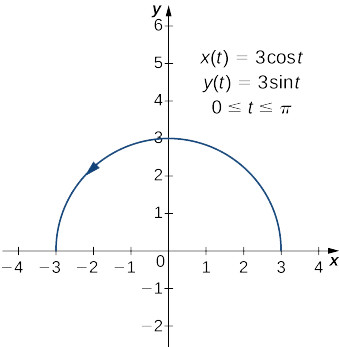
Find the arc length of the semicircle defined by the equations
x(t)=3\cos t, \quad y(t)=3\sin t, \quad \text{for }0≤t≤π. \nonumber
Solution
The values t=0 to t=π trace out the blue curve in Figure \PageIndex{8}. To determine its length, use Equation \ref{arcP}:
\begin{align*} s &=\int^{t_2}_{t_1}\sqrt{\left(\dfrac{dx}{dt}\right)^2+\left(\dfrac{dy}{dt}\right)^2}\,dt\\[4pt] &=\int^π_0\sqrt{(−3\sin t)^2+(3\cos t)^2}\,dt\\[4pt] &=\int^π_0\sqrt{9\sin^2t+9\cos^2t}\,dt\\[4pt] &=\int^π_0\sqrt{9(\sin^2t+\cos^2t)}\,dt\\[4pt] &=\int^π_03\,dt=3t\Big|^π_0\\[4pt] &=3π \text{ units}. \end{align*}
Note that the formula for the arc length of a semicircle is πr and the radius of this circle is 3. This is a great example of using calculus to derive a known formula of a geometric quantity.
Find the arc length of the curve defined by the equations
x(t)=3t^2, \quad y(t)=2t^3, \quad \text{for }1≤t≤3. \nonumber
- Hint
-
Use Equation \ref{arcP}.
- Answer
-
s=2(10^{3/2}−2^{3/2})≈57.589 units
We now return to the problem posed at the beginning of the section about a baseball leaving a pitcher’s hand. Ignoring the effect of air resistance (unless it is a curve ball!), the ball travels a parabolic path. Assuming the pitcher’s hand is at the origin and the ball travels left to right in the direction of the positive x-axis, the parametric equations for this curve can be written as
x(t)=140t, \quad y(t)=−16t^2+2t \nonumber
where t represents time. We first calculate the distance the ball travels as a function of time. This distance is represented by the arc length. We can modify the arc length formula slightly. First rewrite the functions x(t) and y(t) using v as an independent variable, so as to eliminate any confusion with the parameter t:
x(v)=140v, \quad y(v)=−16v^2+2v. \nonumber
Then we write the arc length formula as follows:
\begin{align*} s(t) &=\int^t_0\sqrt{(\dfrac{dx}{dv})^2+(\dfrac{dy}{dv})^2}\,dv\\[4pt] &=\int^t_0\sqrt{140^2+(−32v+2)^2}\,dv \end{align*}
The variable v acts as a dummy variable that disappears after integration, leaving the arc length as a function of time t. To integrate this expression we can use a formula from Appendix A,
\int\sqrt{a^2+u^2}\,du=\dfrac{u}{2}\sqrt{a^2+u^2}+\dfrac{a^2}{2}\ln ∣u+\sqrt{a^2+u^2}∣+C. \nonumber
We set a=140 and u=−32v+2. This gives du=−32\,dv, so dv=−\dfrac{1}{32}\,du. Therefore
\begin{align*} \int\sqrt{140^2+(−32v+2)^2}\,dv &=−\dfrac{1}{32}\int\sqrt{a^2+u^2}\,du\\[4pt] &=−\dfrac{1}{32}\left[\dfrac{(−32v+2)}{2}\sqrt{140^2+(−32v+2)^2}+\dfrac{140^2}{2}\ln ∣(−32v+2)+\sqrt{140^2+(−32v+2)^2}|+C\right] \end{align*}
and
\begin{align*} s(t) &=-\dfrac{1}{32}\left[\dfrac{(-32t+2)}{2}\sqrt{140^2+(-32t+2)^2}+\dfrac{140^2}{2}\ln \left |(-32t+2)+\sqrt{140^2+(-32t+2)^2}\right |\right] +\dfrac{1}{32}\left[\sqrt{140^2+2^2}+\dfrac{140^2}{2}\ln \left |2+\sqrt{140^2+2^2}\right |\right] \\[4pt] &=\left(\dfrac{t}{2}-\dfrac{1}{32}\right)\sqrt{1024t^2-128t+19604}-\dfrac{1225}{4}\ln \left |(-32t+2)+\sqrt{1024t^2-128t+19604}\right |+\dfrac{\sqrt{19604}}{32}+\dfrac{1225}{4}\ln (2+\sqrt{19604}) \end{align*}. \nonumber
This function represents the distance traveled by the ball as a function of time. To calculate the speed, take the derivative of this function with respect to t. While this may seem like a daunting task, it is possible to obtain the answer directly from the Fundamental Theorem of Calculus:
\dfrac{d}{dx}\int^x_af(u)\,du=f(x). \nonumber
Therefore
\begin{align*} s′(t) &= \dfrac{d}{dt}\Big[s(t)\Big]\\[4pt] &=\dfrac{d}{dt}\left[\int^t_0\sqrt{140^2+(−32v+2)^2}\,dv\right]\\[4pt] &=\sqrt{140^2+(−32t+2)^2}\\[4pt] &=\sqrt{1024t^2−128t+19604}\\[4pt] &=2\sqrt{256t^2−32t+4901}. \end{align*} \nonumber
One third of a second after the ball leaves the pitcher’s hand, the distance it travels is equal to
\begin{align*} s\left(\frac{1}{3}\right) &=\left(\frac{1/3}{2}−\frac{1}{32}\right)\sqrt{1024\left(\frac{1}{3}\right)^2−128\left(\frac{1}{3}\right)+19604}\\ &−\frac{1225}{4}\ln \Bigg|\left(−32\left(\frac{1}{3}\right)+2\right)+\sqrt{1024\left(\frac{1}{3}\right)^2−128\left(\frac{1}{3}\right)+19604}\Bigg|\\ &+\frac{\sqrt{19604}}{32}+\frac{1225}{4}\ln(2+\sqrt{19604})\\[4pt] &≈46.69 \text{ feet}.\end{align*}
This value is just over three quarters of the way to home plate. The speed of the ball is
s′\left(\frac{1}{3}\right)=2\sqrt{256\left(\frac{1}{3}\right)^2−32\left(\frac{1}{3}\right)+4901}≈140.27 ft/s.
This speed translates to approximately 95 mph—a major-league fastball.
Surface Area Generated by a Parametric Curve
Recall the problem of finding the surface area of a volume of revolution. In Curve Length and Surface Area, we derived a formula for finding the surface area of a volume generated by a function y=f(x) from x=a to x=b, revolved around the x-axis:
S=2π\int^b_af(x)\sqrt{1+(f′(x))^2}\,dx. \nonumber
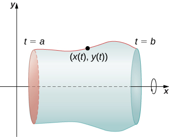
We now consider a volume of revolution generated by revolving a parametrically defined curve x=x(t), \quad y=y(t), \quad \text{for }a≤t≤b around the x-axis as shown in Figure \PageIndex{9}.
The analogous formula for a parametrically defined curve is
S=2π\int^b_ay(t)\sqrt{(x′(t))^2+(y′(t))^2}\,dt \label{ParSurface}
provided that y(t) is not negative on [a,b].
Find the surface area of a sphere of radius r centered at the origin.
Solution
We start with the curve defined by the equations
x(t)=r\cos t, \quad y(t)=r\sin t, \quad \text{for }0≤t≤π. \nonumber
This generates an upper semicircle of radius r centered at the origin as shown in the following graph.
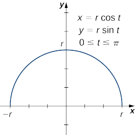
When this curve is revolved around the x-axis, it generates a sphere of radius r. To calculate the surface area of the sphere, we use Equation \ref{ParSurface}:
\begin{align*} S &= 2π\int^b_ay(t)\sqrt{(x′(t))^2+(y′(t))^2}\,dt\\[4pt] &=2π\int^π_0r\sin t\sqrt{(−r\sin t)^2+(r\cos t)^2}\,dt\\[4pt] &=2π\int^π_0r\sin t\sqrt{r^2\sin^2t+r^2\cos^2t}\,dt\\[4pt] &=2π\int^π_0r\sin t\sqrt{r^2(\sin^2t+\cos^2t)}\,dt\\[4pt] &=2π\int^π_0r^2\sin t\,dt\\[4pt] &=2πr^2\left(−\cos t\Big|^π_0\right)\\[4pt] &=2πr^2(−\cos π+\cos 0)\\[4pt] &=4πr^2 \text{ units}^2.\end{align*} \nonumber
This is, in fact, the formula for the surface area of a sphere.
Find the surface area generated when the plane curve defined by the equations
x(t)=t^3, \quad y(t)=t^2, \quad \text{for }0≤t≤1 \nonumber
is revolved around the x-axis.
- Hint
-
Use Equation \ref{ParSurface}. When evaluating the integral, use a u-substitution.
- Answer
-
A=\dfrac{π(494\sqrt{13}+128)}{1215} \text{ units}^2
Key Concepts
- The derivative of the parametrically defined curve x=x(t) and y=y(t) can be calculated using the formula \dfrac{dy}{dx}=\dfrac{y′(t)}{x′(t)}. Using the derivative, we can find the equation of a tangent line to a parametric curve.
- The area between a parametric curve and the x-axis can be determined by using the formula \displaystyle A=\int^{t_2}_{t_1}y(t)x′(t)\,dt.
- The arc length of a parametric curve can be calculated by using the formula s=\int^{t_2}_{t_1}\sqrt{\left(\dfrac{dx}{dt}\right)^2+\left(\dfrac{dy}{dt}\right)^2}\,dt. \nonumber
- The surface area of a volume of revolution revolved around the x-axis is given by S=2π\int^b_ay(t)\sqrt{(x′(t))^2+(y′(t))^2}\,dt. \nonumber
- If the curve is revolved around the y-axis, then the formula is S=2π\int^b_a x(t)\sqrt{(x′(t))^2+(y′(t))^2}\,dt. \nonumber
Key Equations
- Derivative of parametric equations
\dfrac{dy}{dx}=\dfrac{dy/dt}{dx/dt}=\dfrac{y′(t)}{x′(t)} \nonumber
- Second-order derivative of parametric equations
\dfrac{d^2y}{dx^2}=\dfrac{d}{dx}\left(\dfrac{dy}{dx}\right)=\dfrac{(d/dt)(dy/dx)}{dx/dt} \nonumber
- Area under a parametric curve
A=\int^b_ay(t)x′(t)\,dt \nonumber
- Arc length of a parametric curve
s=\int^{t_2}_{t_1}\sqrt{\left(\dfrac{dx}{dt}\right)^2+\left(\dfrac{dy}{dt}\right)^2}\,dt \nonumber
- Surface area generated by a parametric curve
S=2π\int^b_ay(t)\sqrt{(x′(t))^2+(y′(t))^2}\,dt \nonumber