
2.4: Infinite Limits
- Page ID
- 20567
\( \newcommand{\vecs}[1]{\overset { \scriptstyle \rightharpoonup} {\mathbf{#1}} } \)
\( \newcommand{\vecd}[1]{\overset{-\!-\!\rightharpoonup}{\vphantom{a}\smash {#1}}} \)
\( \newcommand{\id}{\mathrm{id}}\) \( \newcommand{\Span}{\mathrm{span}}\)
( \newcommand{\kernel}{\mathrm{null}\,}\) \( \newcommand{\range}{\mathrm{range}\,}\)
\( \newcommand{\RealPart}{\mathrm{Re}}\) \( \newcommand{\ImaginaryPart}{\mathrm{Im}}\)
\( \newcommand{\Argument}{\mathrm{Arg}}\) \( \newcommand{\norm}[1]{\| #1 \|}\)
\( \newcommand{\inner}[2]{\langle #1, #2 \rangle}\)
\( \newcommand{\Span}{\mathrm{span}}\)
\( \newcommand{\id}{\mathrm{id}}\)
\( \newcommand{\Span}{\mathrm{span}}\)
\( \newcommand{\kernel}{\mathrm{null}\,}\)
\( \newcommand{\range}{\mathrm{range}\,}\)
\( \newcommand{\RealPart}{\mathrm{Re}}\)
\( \newcommand{\ImaginaryPart}{\mathrm{Im}}\)
\( \newcommand{\Argument}{\mathrm{Arg}}\)
\( \newcommand{\norm}[1]{\| #1 \|}\)
\( \newcommand{\inner}[2]{\langle #1, #2 \rangle}\)
\( \newcommand{\Span}{\mathrm{span}}\) \( \newcommand{\AA}{\unicode[.8,0]{x212B}}\)
\( \newcommand{\vectorA}[1]{\vec{#1}} % arrow\)
\( \newcommand{\vectorAt}[1]{\vec{\text{#1}}} % arrow\)
\( \newcommand{\vectorB}[1]{\overset { \scriptstyle \rightharpoonup} {\mathbf{#1}} } \)
\( \newcommand{\vectorC}[1]{\textbf{#1}} \)
\( \newcommand{\vectorD}[1]{\overrightarrow{#1}} \)
\( \newcommand{\vectorDt}[1]{\overrightarrow{\text{#1}}} \)
\( \newcommand{\vectE}[1]{\overset{-\!-\!\rightharpoonup}{\vphantom{a}\smash{\mathbf {#1}}}} \)
\( \newcommand{\vecs}[1]{\overset { \scriptstyle \rightharpoonup} {\mathbf{#1}} } \)
\( \newcommand{\vecd}[1]{\overset{-\!-\!\rightharpoonup}{\vphantom{a}\smash {#1}}} \)
\(\newcommand{\avec}{\mathbf a}\) \(\newcommand{\bvec}{\mathbf b}\) \(\newcommand{\cvec}{\mathbf c}\) \(\newcommand{\dvec}{\mathbf d}\) \(\newcommand{\dtil}{\widetilde{\mathbf d}}\) \(\newcommand{\evec}{\mathbf e}\) \(\newcommand{\fvec}{\mathbf f}\) \(\newcommand{\nvec}{\mathbf n}\) \(\newcommand{\pvec}{\mathbf p}\) \(\newcommand{\qvec}{\mathbf q}\) \(\newcommand{\svec}{\mathbf s}\) \(\newcommand{\tvec}{\mathbf t}\) \(\newcommand{\uvec}{\mathbf u}\) \(\newcommand{\vvec}{\mathbf v}\) \(\newcommand{\wvec}{\mathbf w}\) \(\newcommand{\xvec}{\mathbf x}\) \(\newcommand{\yvec}{\mathbf y}\) \(\newcommand{\zvec}{\mathbf z}\) \(\newcommand{\rvec}{\mathbf r}\) \(\newcommand{\mvec}{\mathbf m}\) \(\newcommand{\zerovec}{\mathbf 0}\) \(\newcommand{\onevec}{\mathbf 1}\) \(\newcommand{\real}{\mathbb R}\) \(\newcommand{\twovec}[2]{\left[\begin{array}{r}#1 \\ #2 \end{array}\right]}\) \(\newcommand{\ctwovec}[2]{\left[\begin{array}{c}#1 \\ #2 \end{array}\right]}\) \(\newcommand{\threevec}[3]{\left[\begin{array}{r}#1 \\ #2 \\ #3 \end{array}\right]}\) \(\newcommand{\cthreevec}[3]{\left[\begin{array}{c}#1 \\ #2 \\ #3 \end{array}\right]}\) \(\newcommand{\fourvec}[4]{\left[\begin{array}{r}#1 \\ #2 \\ #3 \\ #4 \end{array}\right]}\) \(\newcommand{\cfourvec}[4]{\left[\begin{array}{c}#1 \\ #2 \\ #3 \\ #4 \end{array}\right]}\) \(\newcommand{\fivevec}[5]{\left[\begin{array}{r}#1 \\ #2 \\ #3 \\ #4 \\ #5 \\ \end{array}\right]}\) \(\newcommand{\cfivevec}[5]{\left[\begin{array}{c}#1 \\ #2 \\ #3 \\ #4 \\ #5 \\ \end{array}\right]}\) \(\newcommand{\mattwo}[4]{\left[\begin{array}{rr}#1 \amp #2 \\ #3 \amp #4 \\ \end{array}\right]}\) \(\newcommand{\laspan}[1]{\text{Span}\{#1\}}\) \(\newcommand{\bcal}{\cal B}\) \(\newcommand{\ccal}{\cal C}\) \(\newcommand{\scal}{\cal S}\) \(\newcommand{\wcal}{\cal W}\) \(\newcommand{\ecal}{\cal E}\) \(\newcommand{\coords}[2]{\left\{#1\right\}_{#2}}\) \(\newcommand{\gray}[1]{\color{gray}{#1}}\) \(\newcommand{\lgray}[1]{\color{lightgray}{#1}}\) \(\newcommand{\rank}{\operatorname{rank}}\) \(\newcommand{\row}{\text{Row}}\) \(\newcommand{\col}{\text{Col}}\) \(\renewcommand{\row}{\text{Row}}\) \(\newcommand{\nul}{\text{Nul}}\) \(\newcommand{\var}{\text{Var}}\) \(\newcommand{\corr}{\text{corr}}\) \(\newcommand{\len}[1]{\left|#1\right|}\) \(\newcommand{\bbar}{\overline{\bvec}}\) \(\newcommand{\bhat}{\widehat{\bvec}}\) \(\newcommand{\bperp}{\bvec^\perp}\) \(\newcommand{\xhat}{\widehat{\xvec}}\) \(\newcommand{\vhat}{\widehat{\vvec}}\) \(\newcommand{\uhat}{\widehat{\uvec}}\) \(\newcommand{\what}{\widehat{\wvec}}\) \(\newcommand{\Sighat}{\widehat{\Sigma}}\) \(\newcommand{\lt}{<}\) \(\newcommand{\gt}{>}\) \(\newcommand{\amp}{&}\) \(\definecolor{fillinmathshade}{gray}{0.9}\)Infinite Limits
Evaluating the limit of a function at a point or evaluating the limit of a function from the right and left at a point helps us to characterize the behavior of a function around a given value. As we shall see, we can also describe the behavior of functions that do not have finite limits.
We now turn our attention to \(h(x)=1/(x−2)^2\), the third and final function introduced at the beginning of this section (see Figure(c)). From its graph we see that as the values of x approach 2, the values of \(h(x)=1/(x−2)^2\) become larger and larger and, in fact, become infinite. Mathematically, we say that the limit of \(h(x)\) as x approaches 2 is positive infinity. Symbolically, we express this idea as
\[\lim_{x \to 2}h(x)=+∞.\]
More generally, we define infinite limits as follows:
Definitions: infinite limits
We define three types of infinite limits.
Infinite limits from the left: Let \(f(x)\) be a function defined at all values in an open interval of the form \((b,a)\).
i. If the values of \(f(x)\) increase without bound as the values of x (where \(x<a\)) approach the number \(a\), then we say that the limit as x approaches a from the left is positive infinity and we write \[\lim_{x \to a−}f(x)=+∞.\]
ii. If the values of \(f(x)\) decrease without bound as the values of x (where \(x<a\)) approach the number \(a\), then we say that the limit as x approaches a from the left is negative infinity and we write \[\lim_{x \to a−}f(x)=−∞.\]
Infinite limits from the right: Let \(f(x)\) be a function defined at all values in an open interval of the form \((a,c)\).
i. If the values of \(f(x)\) increase without bound as the values of x (where \(x>a\)) approach the number \(a\), then we say that the limit as x approaches a from the left is positive infinity and we write \[\lim_{x \to a+}f(x)=+∞.\]
ii. If the values of \(f(x)\) decrease without bound as the values of x (where \(x>a\)) approach the number \(a\), then we say that the limit as x approaches a from the left is negative infinity and we write \[\lim_{x \to a+}f(x)=−∞.\]
Two-sided infinite limit: Let \(f(x)\) be defined for all \(x≠a\) in an open interval containing \(a\)
i. If the values of \(f(x)\) increase without bound as the values of x (where \(x≠a\)) approach the number \(a\), then we say that the limit as x approaches a is positive infinity and we write \[\lim_{x \to a} f(x)=+∞.\]
ii. If the values of \(f(x)\) decrease without bound as the values of x (where \(x≠a\)) approach the number \(a\), then we say that the limit as x approaches a is negative infinity and we write \[\lim_{x \to a}f(x)=−∞.\]
It is important to understand that when we write statements such as \(\displaystyle \lim_{x \to a}f(x)=+∞\) or \(\displaystyle \lim_{x \to a}f(x)=−∞\) we are describing the behavior of the function, as we have just defined it. We are not asserting that a limit exists. For the limit of a function f(x) to exist at a, it must approach a real number L as x approaches a. That said, if, for example, \(\displaystyle \lim_{x \to a}f(x)=+∞\), we always write \(\displaystyle \lim_{x \to a}f(x)=+∞\) rather than \(\displaystyle \lim_{x \to a}f(x)\) DNE.
Example \(\PageIndex{5}\): Recognizing an Infinite Limit
Evaluate each of the following limits, if possible. Use a table of functional values and graph \(f(x)=1/x\) to confirm your conclusion.
- \(\displaystyle \lim_{x \to 0−} \frac{1}{x}\)
- \(\displaystyle \lim_{x \to 0+} \frac{1}{x}\)
- \( \displaystyle \lim_{x \to 0}\frac{1}{x}\)
Solution
Begin by constructing a table of functional values.
| \(x\) | \(\frac{1}{x}\) | \(x\) | \(\frac{1}{x}\) |
|---|---|---|---|
| -0.1 | -10 | 0.1 | 10 |
| -0.01 | -100 | 0.01 | 100 |
| -0.001 | -1000 | 0.001 | 1000 |
| -0.0001 | -10,000 | 0.0001 | 10,000 |
| -0.00001 | -100,000 | 0.00001 | 100,000 |
| -0.000001 | -1,000,000 | 0.000001 | 1,000,000 |
a. The values of \(1/x\) decrease without bound as \(x\) approaches 0 from the left. We conclude that
\[\lim_{x \to 0−}\frac{1}{x}=−∞.\nonumber\]
b. The values of \(1/x\) increase without bound as \(x\) approaches 0 from the right. We conclude that
\[\lim_{x \to 0+}\frac{1}{x}=+∞. \nonumber\]
c. Since \(\displaystyle \lim_{x \to 0−}\frac{1}{x}=−∞\) and \(\displaystyle \lim_{x \to 0+}\frac{1}{x}=+∞\) have different values, we conclude that
\[\lim_{x \to 0}\frac{1}{x}DNE. \nonumber\]
The graph of \(f(x)=1/x\) in Figure \(\PageIndex{8}\) confirms these conclusions.
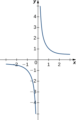
Figure \(\PageIndex{8}\): The graph of \(f(x)=1/x\) confirms that the limit as x approaches 0 does not exist.
Exercise \(\PageIndex{5}\)
Evaluate each of the following limits, if possible. Use a table of functional values and graph \(f(x)=1/x^2\) to confirm your conclusion.
- \(\displaystyle \lim_{x \to 0−}\frac{1}{x^2}\)
- \(\displaystyle \lim_{x \to 0+}\frac{1}{x^2}\)
- \(\displaystyle \lim_{x \to 0}\frac{1}{x^2}\)
Infinite Limits from Positive Integers
If \(n\) is a positive even integer, then
\[\lim_{x \to a}\frac{1}{(x−a)^n}=+∞.\]
If \(n\) is a positive odd integer, then
\[\lim_{x \to a+}\frac{1}{(x−a)^n}=+∞\]
and
\[\lim_{x \to a−}\frac{1}{(x−a)^n}=−∞.\]
We should also point out that in the graphs of \(f(x)=1/(x−a)^n\), points on the graph having x-coordinates very near to a are very close to the vertical line \(x=a\). That is, as \(x\) approaches \(a\), the points on the graph of \(f(x)\) are closer to the line \(x=a\). The line \(x=a\) is called a vertical asymptote of the graph. We formally define a vertical asymptote as follows:
Definition: Vertical Asymptotes
Let \(f(x)\) be a function. If any of the following conditions hold, then the line \(x=a\) is a vertical asymptote of \(f(x)\).
\[\lim_{x \to a−}f(x)=+∞\]
\[\lim_{x \to a−}f(x)=−∞\]
\[\lim_{x \to a+}f(x)=+∞\]
\[\lim_{x \to a+}f(x)=−∞\]
\[\lim_{x \to a}f(x)=+∞\]
\[\lim_{x \to a}f(x)=−∞\]
Example \(\PageIndex{6}\): Finding a Vertical Asymptote
Evaluate each of the following limits using Note. Identify any vertical asymptotes of the function \(f(x)=1/(x+3)^4.\)
- \(\displaystyle \lim_{x \to −3−}\frac{1}{(x+3)^4}\)
- \(\displaystyle \lim_{x \to −3+}\frac{1}{(x+3)^4}\)
- \(\displaystyle \lim_{x \to −3}\frac{1}{(x+3)^4}\)
Solution
We can use Note directly.
- \(\displaystyle \lim_{x \to −3^−}\frac{1}{(x+3)^4}=+∞\)
- \(\displaystyle \lim_{x \to −3^+}\frac{1}{(x+3)^4}=+∞\)
- \(\displaystyle \lim_{x \to −3}\frac{1}{(x+3)^4}=+∞\)
The function \(f(x)=1/(x+3)^4\) has a vertical asymptote of \(x=−3\).
Exercise \(\PageIndex{6}\)
Evaluate each of the following limits. Identify any vertical asymptotes of the function \(f(x)=\frac{1}{(x−2)^3}\).
- \(\displaystyle \lim_{x→2−}\frac{1}{(x−2)^3}\)
- \(\displaystyle \lim_{x→2+}\frac{1}{(x−2)^3}\)
- \(\displaystyle \lim_{x→2}\frac{1}{(x−2)^3}\)
- Answer a
-
\(\displaystyle \lim_{x→2−}\frac{1}{(x−2)^3}=−∞\)
- Answer b
-
\(\displaystyle \lim_{x→2+}\frac{1}{(x−2)^3}=+∞\)
- Answer c
-
\(\displaystyle \lim_{x→2}\frac{1}{(x−2)^3}\) DNE. The line \(x=2\) is the vertical asymptote of \(f(x)=1/(x−2)^3.\)
In the next example we put our knowledge of various types of limits to use to analyze the behavior of a function at several different points.
Example \(\PageIndex{7}\): Behavior of a Function at Different Points
Use the graph of \(f(x)\) in Figure \(\PageIndex{10}\) to determine each of the following values:
- \(\displaystyle \lim_{x \to −4^−}f(x)\);\(\displaystyle \lim_{x \to −4^+}f(x)\); \(\displaystyle\ lim_{x→−4}f(x);f(−4)\)
- \(\displaystyle \lim_{x \to −2^−}f(x\));\(\displaystyle \lim_{x \to −2^+}f(x)\); \(\displaystyle \lim_{x→−2}f(x);f(−2)\)
- \( \displaystyle \lim_{x \to 1^−}f(x)\); \(\displaystyle \lim_{x \to 1+}f(x)\); \(\displaystyle \lim_{x \to 1}f(x);f(1)\)
- \( \displaystyle \lim_{x \to 3^−}f(x)\); \(\displaystyle \lim_{x \to 3+}f(x)\); \(\displaystyle \lim_{x \to 3}f(x);f(3)\)
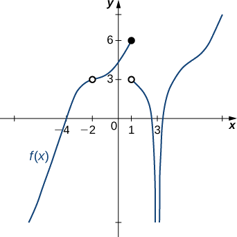
Figure \(\PageIndex{10}\): The graph shows \(f(x)\).
Solution
Using the definitions above and the graph for reference, we arrive at the following values:
- \(\displaystyle \lim_{x \to −4^−}f(x)=0\); \(\displaystyle \lim_{x \to −4^+}f(x)=0\); \(\displaystyle \lim_{x \to −4}f(x)=0;f(−4)=0\)
- \(\displaystyle \lim_{x \to −2^−}f(x)=3\); \(\displaystyle \lim_{x \to −2^+}f(x)=3\); \(\displaystyle \lim_{x \to −2}f(x)=3;f(−2)\) is undefined
- \(\displaystyle \lim_{x \to 1^−}f(x)=6\);\(\displaystyle \lim_{x \to 1^+}f(x)=3\); \(\displaystyle \lim_{x \to 1}f(x)\) DNE; \(f(1)=6\)
- \(\displaystyle \lim_{x \to 3^−}f(x)=−∞\);\(\displaystyle \lim_{x \to 3^+}f(x)=−∞\);\(\displaystyle \lim_{x \to 3}f(x)=−∞\);\(f(3)\) is undefined
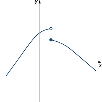
Exercise \(\PageIndex{7}\)
Evaluate \(\displaystyle\lim_{x \to 1}f(x)\) for \(f(x)\) shown here:
- Hint
-
Compare the limit from the right with the limit from the left.
- Answer
-
Does not exist
Example \(\PageIndex{8}\): Einstein’s Equation
In the Chapter opener we mentioned briefly how Albert Einstein showed that a limit exists to how fast any object can travel. Given Einstein’s equation for the mass of a moving object
\[m=\dfrac{m_0}{\sqrt{1−\frac{v^2}{c^2}}}, \nonumber\]
what is the value of this bound?
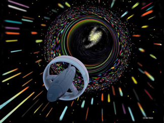
Figure \(\PageIndex{11}\). (Crefit:NASA)
Solution
Our starting point is Einstein’s equation for the mass of a moving object,
\[m=\dfrac{m_0}{\sqrt{1−\frac{v^2}{c^2}}}, \nonumber\]
where \(m_0\) is the object’s mass at rest, \(v\) is its speed, and \(c\) is the speed of light. To see how the mass changes at high speeds, we can graph the ratio of masses \(m/m_0\) as a function of the ratio of speeds, \(v/c\) (Figure \(\PageIndex{11}\)).
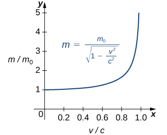
Figure \(\PageIndex{11}\): This graph shows the ratio of masses as a function of the ratio of speeds in Einstein’s equation for the mass of a moving object.
We can see that as the ratio of speeds approaches 1—that is, as the speed of the object approaches the speed of light—the ratio of masses increases without bound. In other words, the function has a vertical asymptote at \(v/c=1\). We can try a few values of this ratio to test this idea.
| \(v/c\) | \(\sqrt{1-\frac{v^2}{c^2}}\) | \(m/m_o\) |
|---|---|---|
| 0.99 | 0.1411 | 7.089 |
| 0.999 | 0.0447 | 22.37 |
| 0.9999 | 0.0141 | 70.7 |
Thus, according to Table \(\PageIndex{3}\):, if an object with mass 100 kg is traveling at 0.9999c, its mass becomes 7071 kg. Since no object can have an infinite mass, we conclude that no object can travel at or more than the speed of light.
Example \(\PageIndex{9}\): Evaluating a Limit of the Form \(K/0,K≠0\) Using the Limit Laws
Evaluate \(\displaystyle \lim_{x→2−}\dfrac{x−3}{x^2−2x}\).
Solution:
Step 1. After substituting in \(x=2\), we see that this limit has the form \(−1/0\). That is, as x approaches 2 from the left, the numerator approaches −1; and the denominator approaches 0. Consequently, the magnitude of \dfrac{x−3}{x(x−2)} becomes infinite. To get a better idea of what the limit is, we need to factor the denominator:
\[\lim_{x→2−}\dfrac{x−3}{x^2−2x}=\lim_{x→2−}\dfrac{x−3}{x(x−2)}.\]
Step 2. Since \(x−2\) is the only part of the denominator that is zero when 2 is substituted, we then separate \(1/(x−2)\) from the rest of the function:
\[=\lim_{x→2^−}\dfrac{x−3}{x}⋅\dfrac{1}{x−2}.\]
Step 3. \(\displaystyle \lim_{x→2^−}\dfrac{x−3}{x}=−\dfrac{1}{2}\) and \(\displaystyle \lim_{x→2^−}\dfrac{1}{x−2}=−∞\). Therefore, the product of \((x−3)/x\) and \(1/(x−2)\) has a limit of \(+∞\):
\[\lim_{x→2^−}\dfrac{x−3}{x^2−2x}=+∞.\]
Exercise \(\PageIndex{9}\)
Evaluate \(\displaystyle \lim_{x→1}\dfrac{x+2}{(x−1)^2}\).
- Solution
-
Use the methods from Example \(\PageIndex{10}\).
- Answer
-
+∞
The Squeeze Theorem
Key Concepts
- A table of values or graph may be used to estimate a limit.
- If the limit of a function at a point does not exist, it is still possible that the limits from the left and right at that point may exist.
- If the limits of a function from the left and right exist and are equal, then the limit of the function is that common value.
- We may use limits to describe infinite behavior of a function at a point.
Key Equations
- Intuitive Definition of the Limit
\(\displaystyle \lim_{x \to a}f(x)=L\)
- Two Important Limits
\(\displaystyle \lim_{x \to a}x=a\) \(\displaystyle \lim_{x \to a}c=c\)
- One-Sided Limits
\(\displaystyle \lim_{x \to a^−}f(x)=L\) \(\displaystyle \lim_{x \to a^+}f(x)=L\)
- Infinite Limits from the Left
\(\displaystyle \lim_{x \to a^−}f(x)=+∞\) \(\displaystyle \lim_{x \to a^−} f(x)=−∞\)
- Infinite Limits from the Right
\(\displaystyle \lim_{x \to a^+}f(x)=+∞\) \(\displaystyle \lim_{x \to a^+} f(x)=−∞\)
- Two-Sided Infinite Limits
\(\displaystyle \lim_{x \to a}f(x)=+∞\): \(\displaystyle \lim_{x \to a^−}f(x)=+∞\) and \(lim_{x \to a^+} f(x)=+∞\)
\(\displaystyle \lim_{x \to a}f(x)=−∞\): \(\displaystyle \lim_{x \to a^−}f(x)=−∞\) and \(lim_{x \to a^+} f(x)=−∞\)
For the following exercises, consider the function \(f(x)=\frac{x^2−1}{|x−1|}.\)
Glossary
- infinite limit
- A function has an infinite limit at a point a if it either increases or decreases without bound as it approaches a
- intuitive definition of the limit
- If all values of the function \(f(x)\) approach the real number L as the values of \(x(≠a)\) approach a, \(f(x)\) approaches L
- one-sided limit
- A one-sided limit of a function is a limit taken from either the left or the right
- vertical asymptote
- A function has a vertical asymptote at \(x=a\) if the limit as x approaches a from the right or left is infinite
Contributors
Gilbert Strang (MIT) and Edwin “Jed” Herman (Harvey Mudd) with many contributing authors. This content by OpenStax is licensed with a CC-BY-SA-NC 4.0 license. Download for free at http://cnx.org.
Follow the procedures from Example \(\PageIndex{4}\).
a. \(\displaystyle \lim_{x \to 0−}\frac{1}{x^2}=+∞\);
b. \(\displaystyle \lim_{x \to 0+}\frac{1}{x^2}=+∞\);
c. \(\displaystyle \lim_{x \to 0}\frac{1}{x^2}=+∞\)