
2.8: Periodic functions and oscillations


- Last updated
- Oct 29, 2020
- Save as PDF
( \newcommand{\kernel}{\mathrm{null}\,}\)
There are many periodic phenomena in the biological sciences. Examples include wingbeat of insects and of birds, nerve action potentials, heart beat, breathing, rapid eye movement sleep, circadian rhythms (sleep-wake cycles), women’s menstrual cycle, bird migrations, measles incidence, locust emergence. All of these examples are periodic repetition with time, the variable usually associated with periodicity. The examples are listed in order of increasing period of repetition in Table 2.8.
| Biological Process | Period | Biological Process | Period |
|---|---|---|---|
| Insect wingbeat | 0.02 sec | Circadian cycle (sleep-wake) | 1 day |
| Nerve action potential | 0.2 sec | Menstrual cycle | 28 days |
| Heart beat | 1 sec | Bird migrations | 1 year |
| Breathing (rest) | 5 sec | Measles | 2 years |
| REM sleep | ≈ 90 min | Locust | 17 years |
| Tides | 6 hours |
A measurement usually quantifies the state of a process periodic with time and defines a function characteristic of the process. Some examples are shown in Figure 2.8.1. The measurement may be of physical character as in electrocardiograms, categorical as in stages of sleep, or biological as in measurement of hormonal level.
There are also periodic variations with space that result in the color patterns on animals – stripes on zebras and tigers, spots on leopards – , regular spacing of nesting sites, muscle striations, segments in a segmented worm, branching in nerve fibers, and the five fold symmetry of echinoderms. Some spatially periodic structures are driven by time-periodic phenomena – branches in a tree, annular tree rings, chambers in a nautilus, ornamentation on a snail shell. The pictures in Figure 2.6.2 illustrate some periodic functions that vary with linear space. The brittle star shown in Figure 2.8.3 varies periodically with angular change in space.
In all instances there is an independent variable, generally time or space, and a dependent variable that is said to be periodic.
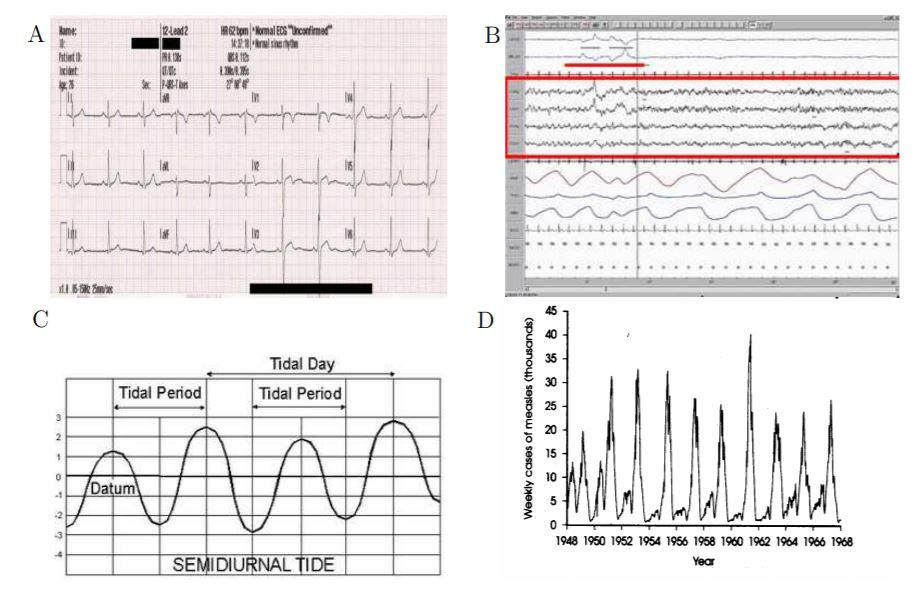
Figure 2.8.1: Figures demonstrating periodic repetition with time. (A) Electorcardiogram. http://en.wikipedia.org/wiki/Electrocardiography uploaded by MoodyGroove. (B) This is a screenshot of a polysomnographic record (30 seconds) representing Rapid Eye Movement Sleep. EEG highlighted by red box. Eye movements highlighted by red line. http://en.wikipedia.org/wiki/File:REM.png uploaded by Mr. Sandman. (C) Tidal movement (≈12 hr) (http://en.wikipedia.org/wiki/Tide), uploaded from NOAA, http://coops.nos.noaa.gov/images/restfig6.gif. (D) Recurrent epidemics of measles (≈2 yr), Anderson and May, Vaccination and herd immunity to infectious diseases, Nature 318 1985, pp 323-9, Figure 1a.
Definition 2.8.1 Periodic Function
A function, F, is said to be periodic if there is a positive number, p, such that for every number x in the domain of F, x+p is also in the domain of F and
F(x+p)=F(x)
and for each number q where 0<q<p there is some x in the domain of F for which
F(x+q)≠F(x)
The period of F is p.
The amplitude of a periodic function F is one-half the difference between the largest and least values of F(t), when these values exist.
The condition that ‘for every number x in the domain of F, x+p is also in the domain of F’ implies that the domain of F is infinite in extent — it has no upper bound. Obviously, all of the examples that we experience are finite in extent and do not satisfy Definition 2.8.1. We will use ‘periodic’ even though we do not meet this requirement.
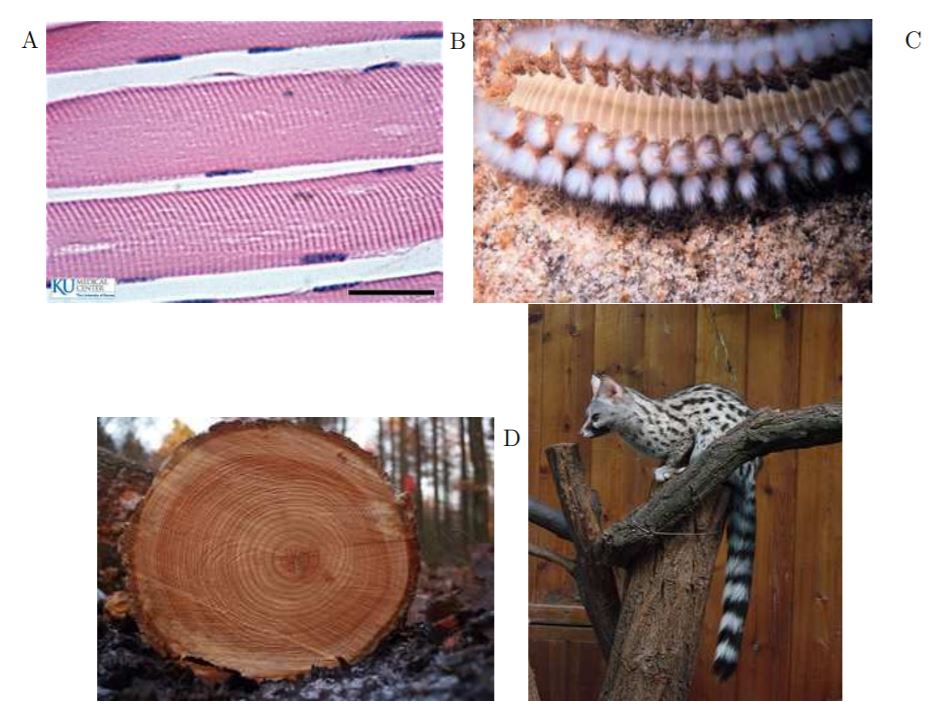
Figure 2.8.2: Figures demonstrating periodic repetition with space. A. Muscle striations, Kansas University Medical School, http://www.kumc.edu/instruction/medicine/anatomy/histoweb/muscular/muscle02.htm. B. Bristle worm, http://www.photolib.noaa.gov/htmls/reef1016.htm Image ID: reef1016, Dr. Anthony R. Picciolo. C. Annular rings, uploaded by Arnoldius to commons.wikimedia.org/wiki D. A common genet (Genetta genetta), http://en.wikipedia.org/wiki/File:Genetta genetta felina (Wroclaw zoo).JPG Uploaded by Gu´erin Nicolas. Note a periodic distribution of spots on the body and stripes on the tail.
examples that we experience are finite in extent and do not satisfy Definition 2.8.1. We will use ‘periodic’ even though we do not meet this requirement.
The condition ‘when these numbers exist’ in the definition of amplitude is technical and illustrated in Figure 2.8.4 by the graph of
F(t)=t−[t]
where [t] denotes the integer part of t. ([π]=3,[√30]=5). There is no largest value of F(t).
F(n)=n−[n]=0 for integer n
If t is such that F(t) is the largest value of F then t is not an integer and is between an integer n and n+1. The midpoint s of [t,n+1] has the property that F(t)<F(s), so that F(t) is not the largest value of F.
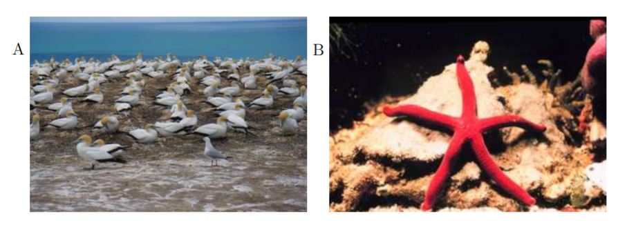
Figure 2.8.3: A. Periodic distribution of Gannet nests in New Zealand. B. A star fish demonstrating angular periodicity, NOAA’s Coral Kingdom Collection, Dr. James P. McVey, http://www.photolib.noaa.gov/htmls/reef0296.htm.
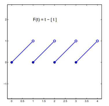
Figure \(\PageIndex{4]\): The graph of F(t)=t−[t] has no highest point.
The function, F(t)=t−[t] is pretty clearly periodic of period 1, and we might say that its amplitude is 0.5 even though it does not satisfy the definition for amplitude. Another periodic function that has no amplitude is the tangent function from trigonometry.
Periodic Extension Periodic functions in nature do not strictly satisfy Definition 2.8.1, but can be approximated with strictly periodic functions over a finite interval of their domain. Periodic functions in nature also seldom have simple equation descriptions. However, one can sometimes describe the function over one period and then assert that the function is periodic – thus describing the entire function.
Example 2.8.1 Electrocardiograms have a very characteristic periodic signal as shown in Figure 2.8.1.
A picture of a typical signal from ‘channel I’ is shown in Figure 2.8.5; the regions of the signal, P-R, QRS, etc. correspond to electrical events in the heart that cause contractions of specific muscles. Is there an equation for such a signal? Yes, a very messy one!
The graph of the following equation is shown in Figure 2.8.5(b). It is similar to the typical electrocardiogram in Figure 2.8.5(a).
H(t)=25000(t+0.05)t(t−0.07)(1+(20t)10)2(2(40t))+0.15⋅2−1600(t+0.175)2+0.25⋅2−900(t−0.2)2−0.4≤t≤0.4
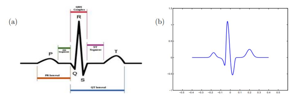
Figure 2.8.5: (a) Typical signal from an electrocardiogram, created by Agateller (Anthony Atkielski) http://en.wikipedia.org/wiki/Electrocardiography, . (b) Graph of Equation 2.12
Explore 2.8.1 Technology Draw the graph of the heart beat Equation 2.12. You will find it useful to break the function into parts. It is useful to define
y1=25000(x+0.05)x(x−0.07)(1+(20x)10)y2=(y1)/2(2(40x))
and y3 and y4 for the other two terms, then combine y2, y3 and y4 into y5 and select only y5 to graph.
The heart beat function H in Equation 2.12 is not a periodic function and is defined only for −0.4≤t≤0.4. Outside that interval, the expression defining H(t) is essentially zero. However, we can simultaneously extend the definition of H and make it periodic by
H(t)=H(t−0.8) for all t
What is the impact of this? H(0.6), say is now defined, to be H(−0.2). Immediately, H has meaning for 0.4≤t≤1.2, and the graph is shown in Figure 2.8.6(a). Now because H(t) has meaning on 0.4≤t≤1.2, H also has meaning on 0.4≤t≤2.0 and the graph is shown in Figure 2.8.6(b). The extension continues indefinitely.
Definition 2.8.2 Periodic extension of a function. If f is a function defined on an interval [a, b) and p = b − a, the periodic extension of F of f is defined by
F(t)=f(t) for a≤t<bF(t+p)=F(t) for −∞<t<∞
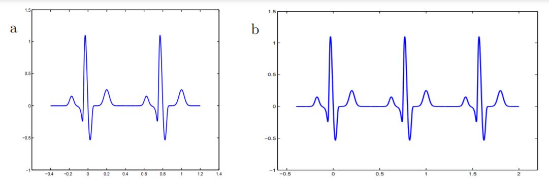
Figure 2.8.6: (a) Periodic extension of the heart beat function H of Equation ??? by one period. (a) Periodic extension of the heart beat function H to two periods.
Equation ??? is used recursively. For t in [a b), t + p is in [b, b + p) and Equation ??? defines F on [b, b + p). Then, for t in [b, b + p), t + p is in [b + p, b + 2p) and Equation ??? defines F on [b + p, b + 2p). Continue this for all values of t > b. If t is in [a − p, a) then t + p is in [a, b) and F(t) = F(t + p). Continuing in this way, F is defined for all t less than a.
Exercises for Section 2.8, Periodic functions and oscillations.
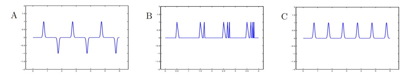
Exercise 2.8.1 Which of the three graphs in Figure Ex. 2.8.1 are periodic. For any that is periodic, find the period and the amplitude.
Figure for Exercise 2.8.1 Three graphs for Exercise 2.8.1 .
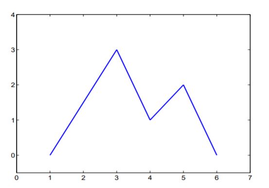
Exercise 2.8.2 Shown in Figure Ex. 2.8.2 is the graph of a function, f defined on the interval [1,6]. Let F be the periodic extension of f.
- What is the period of F?
- Draw a graph of F over three periods.
- Evaluate F(1),F(3),F(8),F(23),F(31) and F(1004).
- Find the amplitude of F.
Figure for Exercise 2.8.2 Graph of a function f for Exercise 2.8.2.
Exercise 2.8.3 Suppose your are traveling an interstate highway and that every 10 miles there is an emergency telephone. Let D be the function defined by
D(x) is the distance to the nearest emergency telephone
where x is the mileage position on the highway.
- Draw a graph of D.
- Find the period and amplitude of D.
Exercise 2.8.4 Your 26 inch diameter bicycle wheel has a patch on it. Let P be the function defined by
P(x) is the distance from patch to the ground
where x is the distance you have traveled on a bicycle trail.
- Draw a graph of P (approximate is acceptable).
- Find the period and amplitude of P.
Exercise 2.8.5 Let F be the function defined for all numbers, x, by
F(x)= the distance from x to the even integer nearest x
- Draw a graph of F.
- Find the period and amplitude of F.
Exercise 2.8.6 Let f be the function defined by
f(x)=1−x2−1≤x≤1
Let F be the extension of f with period 2.
- Draw a graph of f.
- Draw a graph of F.
- Evaluate F(1),F(2),F(3),F(12),F(31) and F(1002).
- Find the amplitude of F.
2.8.1 Trigonometric Functions.
The trigonometric functions are perhaps the most familiar periodic functions and often are used to describe periodic behavior. However, not many of the periodic functions in biology are as simple as the trigonometric functions, even over restricted domains.
Amplitude and period and frequency of a Cosine Function
The function
H(t)=Acos(2πPt+ϕ)A>0P>0
and ϕ any angle has amplitude A, period P, and frequency 1/P.
Graphs of rescaled cosine functions shown in Figure 2.8.7 demonstrate the effects of A and P.
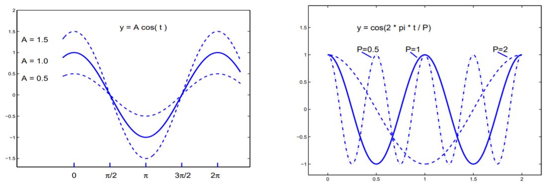
Figure 2.8.7: (a) Graphs of the cosine function for amplitudes 0,5 1.5 and 1.5. (b) Graphs of the cosine function for periods 0.5, 1.0 and 2.0.
Example 2.8.2
Problem. Find the period, frequency, and amplitude of
H(t)=3sin(5t+π/3)
Solution. Write H(t)=3sin(5t+π/3) as
H(t)=3sin(2π2π/5t+π/3)
Then the amplitude of P is 3, and the period is 2π/5 and the frequency is 5/(2π).
Motion of a Spring-Mass System A mass suspended from a spring, when vertically displaced from equilibrium a small amount will oscillate above and below the equilibrium position. A graph of displacement from equilibrium vs time is shown in in Figure 2.8.8A for a certain system. Critical points of the graph are
(2.62s,72.82cm),(3.18s,46.24cm), and (3.79s,72.80cm)
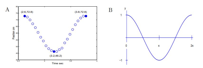
Figure 2.8.8: Graphs of A. the motion of a spring-mass system and B. H(t)=cost.
Also shown is the graph of the cosine function, H(t)=cost.
It is clear that the data and the cosine in Figure 2.8.8 have similar shapes, but examine the axes labels and see that their periods and amplitudes are different and the graphs lie in different regions of the plane. We wish to obtain a variation of the cosine function that will match the data.
The period of the harmonic motion is 3.79−2.62=1.17 seconds, the time of the second peak minus the time of the first peak. The amplitude of the harmonic motion is 0.5(72.82−46.24)=13.29 cm, one-half the difference of the heights of the highest and lowest points.
Now we expect a function of the form
H0(t)=13.3cos(2π1.17t)
to have the shape of the data, but we need to translate vertically and horizontally to match the data. The graphs of H0 and the data are shown in Figure 2.8.9A, and the shapes are similar. We need to match the origin (0,0) with the corresponding point (2.62, 59.5) of the data. We write
H(t)=59.5+13.3cos(2π1.17(t−2.62))
The graphs of H and the data are shown in Figure 2.8.9B and there is a good match.
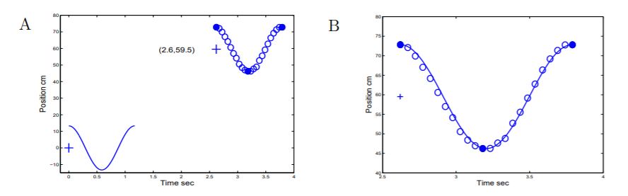
Figure 2.8.9: On the left is the graph of H0(t)=13.3cos(2π1.17t) and the harmonic oscillation data. The two are similar in form. The graph to the right shows the translation, H, of H0, H(t)=59.5+13.3cos(2π1.17(t−2.62)) and its approximation to the harmonic oscillation data.
Polynomial approximations to the sine and cosine functions. Shown in Figure 2.8.10 are the graphs of F(x)=sinx and the graph of (dashed curve)
P3(x)=x−x3120
on [0,π/2].
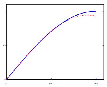
Figure 2.8.10: The graphs of F(x)=sinx (solid) and P3(x)=x−x3120 (dashed) on [0,π/2].
The graph of P3 is hardly distinguishable from the graph of F on the interval [0,π/4], although they do separate near x=π/2. F(x)=sinx is difficult to evaluate (without a calculator) except for special values such as F(0)=sin0=0, F(π/3)=sinπ/3=0.5 and F(π/2)=sinπ/2 = 1.0\). However, P3(x) can be calculated using only multiplication, division and subtraction. The maximum difference between P3 and F on [0,π/4] occurs at π/4 and F(π/4)=sqrt2/2≐0.70711 and P3(π/4)=0.70465. The relative error in using P3(π/4) as an approximation to F(π/4) is
Relative Error =|P3(π/4)−F(π/4)|F(π/4)≐|0.70465−0.70711|0.70711=0.0036
thus less than 0.5% error is made in using the rather simple P3(x)=x−x3120 in place of F(x)=sinx on [0,π/4].
Exercises for Section 2.8.1, Trigonometric functions.
Exercise 2.8.7 Find the periods of the following functions.
- P(t)=sin(π3t)
- P(t)=sin(t)
- P(t)=5−2sin(t)
- P(t)=sin(t)+cos(t)
- P(t)=sin(2π2t)+sin(2π3t)
- P(t)=tan2t
Exercise 2.8.8 Sketch the graphs and label the axes for
(a)y=0.2cos(2π0.8t)and(b)y=5cos(18t+π/6)
Exercise 2.8.9 Describe how the harmonic data of Figure 2.8.9A would be translated so that the graph of the new data would match that of H0.
Exercise 2.8.10 Use the identity, cost=sin(t+π2), to write a sine function that approximates the harmonic oscillation data.
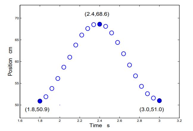
Exercise 2.8.11 Fit a cosine function to the spring-mass oscillation shown in Exercise Figure 2.8.11.
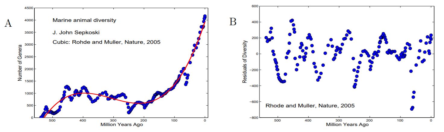
Exercise 2.8.12 A graph of total marine animal diversity over the period from 543 million years ago until today is shown in Exercise Figure 2.8.12A. The data appeared in a paper by Robert A. Rohde and Richard A. Muller5, and are based on work by J. John Sepkoski6. Also shown is a cubic polynomial fit to the data by Robert Rohde and Richard Muller who were interested in the the difference between the data and the cubic shown in Exercise Figure 2.8.12B. They found that a sine function of period 62 million years fit the residuals rather well. Find an equation of such a sine function.
Figure for Exercise 2.8.12 A. Marine animal diversity and a cubic polynomial fit to the data. B. The residuals of the cubic fit. Figures adapted from Robert A. Rohde and Richard A. Muller, Cycles in fossil diversity, Nature 434, 208-210, Copyright 2005, http://www.nature.com
Exercise 2.8.13 Technology Draw the graphs of F(x)=sinx and
F(x)=sinx and P5(x)=x−x36+x5120
on the range 0≤x≤π. Compute the relative error in P5(π/4) as an approximation to F(π/4) and in P5(π/2) as an approximation to F(π/2).
Exercise 2.8.14 Technology Polynomial approximations to the cosine function.
- Draw the graphs of F(x)=cosx and F(x)=cosx and P2(x)=1−x22 on the range 0≤x≤π.
- Compute the relative error in P2(π/4) as an approximation to F(π/4) and in P2(π/2) as an approximation to F(π/2).
- Use a graphing calculator to draw the graphs of F(x)=cosx and P4(x)=1−x22+x424 on the range 0≤x≤π.
- Compute the relative error in P4(π/4) as an approximation to F(π/4) and the absolute error in P4(π/2) as an approximation to F(π/2).
5 Robert A. Rohde and Richard A. Muller, Cycles in fossil diversity, Nature 434, 208-210.
6 J. John Sepkoski, A compendium of Fossil Marine Animal Genera, Eds David Jablonski and Michael Foote, Bulletins of American Paleontology, 363, 2002.