
3.6: Vectors from an Algebraic Point of View


- Last updated
- Jan 2, 2021
- Save as PDF

( \newcommand{\kernel}{\mathrm{null}\,}\)
Focus Questions
The following questions are meant to guide our study of the material in this section. After studying this section, we should understand the concepts motivated by these questions and be able to write precise, coherent answers to these questions.
- How do we find the component form of a vector?
- How do we find the magnitude and the direction of a vector written in component form?
- How do we add and subtract vectors written in component form and how do we find the scalar product of a vector written in component form?
- What is the dot product of two vectors?
- What does the dot product tell us about the angle between two vectors?
- How do we find the projection of one vector onto another?
Introduction and Terminology
We have seen that a vector is completely determined by magnitude and direction. So two vectors that have the same magnitude and direction are equal. That means that we can position our vector in the plane and identify it in different ways. For one, we can place the tip of a vector v at the origin and the tail will wind up at some point (v1,v2) as illustrated in Figure 3.6.1.
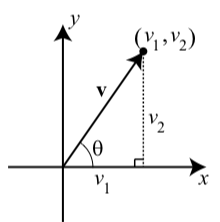
Figure 3.6.1: A Vector in Standard Position
A vector with its initial point at the origin is said to be in standard position and is represent by v=⟨v1,v2⟩. Please note the important distinction in notation between the vector v=⟨v1,v2⟩ and the point (v1,v2). The coordinates of the terminal point (v1,v2) are called the components of the vector v. We call v=⟨v1,v2⟩ the component form of the vector v. The first coordinate v1 is called the x-component or the horizontal component of the vector v, and the first coordinate v2 is called the y-component or the vertical component of the vector v. The nonnegative angle θ between the vector and the positive x-axis (with 0≤θ≤360∘) is called the direction angle of the vector. See Figure 3.6.1.
Using Basis Vectors
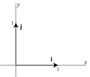
There is another way to algebraically write a vector if the components of the vector are known. This uses the so-called standard basis vectors for vectors in the plane. These two vectors are denoted by i and j and are defined as follows and are shown in the diagram below.
i=⟨1,0⟩ and j=⟨0,1⟩
The diagram in Figure 3.28 shows how to use the vectors i and j to represent a vector v=⟨a,b⟩.
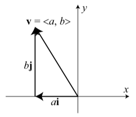
Figure 3.6.2: Using the Vectors i and j
The diagram shows that if we place the base of the vector j at the tip of the vector i, we see that v=⟨a,b⟩=ai+bj
This is often called the i, j form of a vector, and the real number a is called the i-component of v and the real number b is called the j-component of v
Algebraic Formulas for Geometric Properties of a Vector
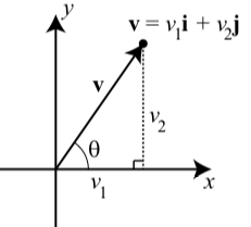
Vectors have certain geometric properties such as length and a direction angle. With the use of the component form of a vector, we can write algebraic formulas for these properties. We will use the diagram to the right to help explain these formulas.
- The magnitude (or length) of the vector v is the distance from the origin to the point (v1,v2) and so |v|=√v21+v22
- The direction angle of v is, where 0≤θ<360∘, and cos(θ)=v1|v| and sin(θ)=v2|v|
- The horizontal and component and vertical component of the vector v and direction angle θ are v1=|v|cos(θ) and v2=|v|sin(θ)
Exercise 3.6.1
- Suppose the horizontal component of a vector v is 7 and the vertical component is −3. So we have v=7i+(−3)j=7i−3j. Determine the magnitude and the direction angle of v.
- Suppose a vector w has a magnitude of 20 and a direction angle of −200∘. Determine the horizontal and vertical components of w and write w in i, j form.
- Answer
-
1. v=7i+(−3)j. So |v|=√72+(−3)2=√58. In addition, cos(θ)=7√58 and sin(θ)=−3√58
So the terminal side of θ is in the fourth quadrant, and we can write θ=360∘−arccos(7√58). So θ≈336.80∘.
2. We are given |w|=20 and the direction angle θ of w is 200∘. So if we write w=w1i+w2j. Then
w1=20cos(200∘)≈−1.794
w1=20cos(200∘)≈−6.840
Operations on Vectors
In Section 3.5, we learned how to add two vectors and how to multiply a vector by a scalar. At that time, the descriptions of these operations was geometric in nature. We now know about the component form of a vector. So a good question is, “Can we use the component form of vectors to add vectors and multiply a vector by a scalar?”
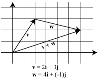
To illustrate the idea, we will look at Progress Check 3.25 on page 223, where we added two vectors v and w. Although we did not use the component forms of these vectors, we can now see that v=⟨2,3⟩=2i+3j and w=⟨4,−1⟩=4i+(−1)j
The diagram above was part of the solutions for this progress check but now shows the vectors in a coordinate plane.
Notice that v+w=6i+2j v+w=(2+4)i+(3+(−1))j
Figure 3.29 shows a more general diagram with v=⟨a,b⟩=ai+bj and w=⟨c,d⟩=ci+dj
in standard position. This diagram shows that the terminal point of v+w in standard position is (a+c,b+d) and so
v+w=⟨a+c,b+d⟩=(a+c)i+(b+d)j
This means that we can add two vectors by adding their horizontal components and by adding their vertical components. The next progress check will illustrate something similar for scalar multiplication.
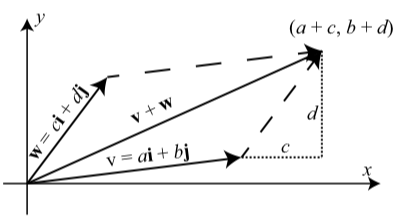
Figure 3.6.3: The Sum of Two Vectors
Exercise 3.6.2
Let v=⟨3,−2⟩. Draw the vector v in standard position and then draw the vectors 2v and −2v in standard position. What are the component forms of the vectors 2v and −2v?
In general, how do you think a scalar multiple of a vector a=⟨a1,a2⟩ by a scalar c should be defined? Write a formal definition of a scalar multiple of a vector based on your intuition.
- Answer
-
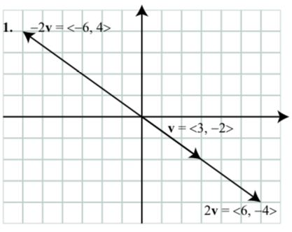
2. For a vector a=⟨a1,a2⟩ and a scalar c, we define the scalar multiple ca to be ca=⟨ca1,ca2⟩.
Based on the work we have done, we make the following formal definitions.
Definition
For vectors v=⟨v1,v2⟩=v1i+v2j and w=⟨w1,w2⟩=w1i+w2j and scalar c, we make the following definition:
v+w=⟨v1+w1,v2+w2⟩
v+w=(v1+w1)i+(v2+w2)j
v−w=⟨v1−w1,v2−w2⟩
v−w=(v1−w1)i+(v2−w2)j
cv=⟨cv1,cv2⟩
cv=(cv1)i+(cv2)j
Exercise 3.6.3
Let u=⟨1,−2⟩, u=⟨0,4⟩, and u=⟨−5,7⟩.
- Determine the component form of the vector 2u−3v.
- Determine the magnitude and the direction angle for 2u−3v.
- Determine the component form of the vector uu+2v−7w.
- Answer
-
Let u=⟨1,−2⟩, and w=⟨−5,7⟩.
1. 2u−3v=⟨2,−4⟩−⟨0,12⟩=⟨2,−16⟩
2. |2u−3v|=√22+(−16)2=√260. So now let θ be the direction angle of 2u−3v. Then
cos(θ)=2√260 and sin(θ)=−16√260.
So the terminal side of θ is in the fourth quadfrant. We see that arcsin(−16√260)≈−82.87∘. Since the direction angle θ must satisfy a≤θ<360circ, we see that θ≈−82.87∘+360∘≈277.13∘.
3. u+2v−7w=⟨1,−2⟩+⟨0,8⟩−⟨−35,49⟩=⟨36,−43⟩.
The Dot Product of Two Vectors
Finding optimal solutions to systems is an important problem in applied mathematics. It is often the case that we cannot find an exact solution that satisfies certain constraints, so we look instead for the “best” solution that satisfies the constraints. An example of this is fitting a least squares curve to a set of data like our calculators do when computing a sine regression curve. The dot product is useful in these situations to find “best” solutions to certain types of problems. Although we won’t see it in this course, having collections of perpendicular vectors is very important in that it allows for fast and efficient computations. The dot product of vectors allows us to measure the angle between them and thus determine if the vectors are perpendicular. The dot product has many applications, e.g., finding components of forces acting in different directions in physics and engineering. We introduce and investigate dot products in this section.
We have seen how to add vectors and multiply vectors by scalars, but we have not yet introduced a product of vectors. In general, a product of vectors should give us another vector, but there turns out to be no really useful way to define such a product of vectors. However, there is a dot “product” of vectors whose output is a scalar instead of a vector, and the dot product is a very useful product (even though it isn’t a product of vectors in a technical sense).
Recall that the magnitude (or length) of the vector u=⟨u1,u2⟩ is: |u|=√u21+u22=√u1u1+u2u2
The expression under the second square root is an important one and we extend it and give it a special name.
Definition
Let u=⟨u1,u2⟩ and v=⟨v1,v2⟩ be vectors in the plane. The dot product of u and v is the scalar u⋅v=u1v1+u2v2.
This may seem like a strange number to compute, but it turns out that the dot product of two vectors is useful in determining the angle between two vectors. Recall that in Progress Check 3.27 on page 225, we used the Law of Cosines to determine the sum of two vectors and then used the Law of Sines to determine the angle between the sum and one of those vectors. We have now seen how much easier it is to compute the sum of two vectors when the vectors are in component form. The dot product will allow us to determine the cosine of the angle between two vectors in component form. This is due to the following result:
The Dot Product and the Angle between Two Vectors
If θ is the angle between two nonzero vectors u and v (0∘≤θ≤180∘), then
u⋅v=|u||v|cos(θ) or cos(θ)=u⋅v|u||v|
Notice that if we have written the vectors v and w in component form, then we have formulas to compute |v|,|w|, and v⋅w. This result may seem surprising but it is a fairly direct consequence of the Law of Cosines as we will now show. Let θ be the angle between u and v as illustrated in Figure 3.30.
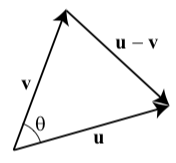
Figure 3.6.4: The angle between u and v
We can apply the Law of Cosines to determine the angle θ as follows:
|u−v|2=|u|2+|v|2−2|u||v|cos(θ)
(u−v)⋅(u−v)=|u|2+|v|2−2|u||v|cos(θ)
(u⋅u)−2(u⋅v)+(v⋅v)=|u|2+|v|2−2|u||v|cos(θ)
|u|2−2(u⋅v)+|v|2=|u|2+|v|2−2|u||v|cos(θ)
−2(u⋅u)=−2|u||v|cos(θ)
u⋅u=|u||v|cos(θ)
Exercise 3.6.4
1. Determine the angle θ between the vectors u=3i+j and v=−5i+2j.
2. Determine all vectors perpendicular to u=⟨1,3⟩. How many such vectors are there? Hint: Let v=⟨a,b⟩. Under what conditions will the angle between u and v be 90∘?
- Answer
-
1. If θ is the angle between u=3i+j and v=−5i+2j, then
cos(θ)=u⋅v|u||v|=−13√10√29
θ=cos−1(−13√10√29)
so θ≈139.764∘.
2. If v=⟨a,b⟩ is perpendicular to u=⟨1,3⟩, then the angle θ between them is 90∘ and so cos(θ)=0. So we must have u⋅v=0 and this means that a+3b=0. So any vector v=⟨a,b⟩ where a=−3b will be perpendicular to v, and there are infinitely many such vectors. One vector perpendicular to u is ⟨−3,1⟩.
One purpose of Progress Check 3.34 was to use the formula cos(θ)=u⋅v|u||v|
to determine when two vectors are perpendicular. Two vectors u and v will be perpendicular if and only if the angle θ between them is 90∘. Since cos(90∘)=0, we see that this formula implies that u and v will be perpendicular if and only if u⋅v=0 (This is because a fraction will be equal to 0 only when the numerator is equal to 0 and the denominator is not zero.) So we have:
Two vectors are perpendicular if and only if their dot product is equal to 0.
Note
When two vectors are perpendicular, we also say that they are orthogonal.
Projections
Another useful application of the dot product is in finding the projection of one vector onto another. An example of where such a calculation is useful is the following.
Usain Bolt from Jamaica excited the world of track and field in 2008 with his world record performances on the track. Bolt won the 100 meter race in a world record time of 9.69 seconds. He has since bettered that time with a race of 9.58 seconds with a wind assistance of 0.9 meters per second in Berlin on August 16, 20092. The wind assistance is a measure of the wind speed that is helping push the runners down the track. It is much easier to run a very fast race if the wind is blowing hard in the direction of the race. So that world records aren’t dependent on the weather conditions, times are only recorded as record times if the wind aiding the runners is less than or equal to 2 meters per second. Wind speed for a race is recorded by a wind gauge that is set up close to the track. It is important to note, however, that weather is not always as cooperative as we might like. The wind does not always blow exactly in the direction of the track, so the gauge must account for the angle the wind makes with the track.
If the wind is blowing in the direction of the vector u and the track is in the direction of the vector v in Figure 3.31, then only part of the total wind vector is actually working to help the runners.
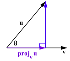
Figure 3.6.5: The Projection of u onto v
This part is called the projection of the vector u onto the vector v and is denoted projvu.
We can find this projection with a little trigonometry. To do so, we let θ be the angle between u and v as shown in Figure 3.6.5. Using right triangle trigonometry, we see that |projvu|=|u|cos(θ)=|u|u⋅v|u||v|=u⋅v|v|
The quantity we just derived is called the scalar projection (or component) of u onto v and is denoted by compvu. Thus compvu=u⋅v|v|
This gives us the length of the vector projection. So to determine the vector, we use a scalar multiple of this length times a unit vector in the same direction, which is 1|v|v. So we obtain
projvu=|projvu|(1|v|)=u⋅v|v|(1|v|)=u⋅v|v|2v
We can also write the projection of u onto v as
projvu=u⋅v|v|2v=u⋅vv⋅vv
The wind component that acts perpendicular to the direction of v in Figure 3.6.5 is called the projection of u orthogonal to v and is denoted proj⊥vu as shown in Figure 3.32. Since u=proj⊥vu+projvu, we have that
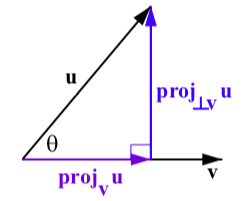
Figure 3.6.6: The Projection of u onto v
proj⊥vu=u−projvu
Following is a summary of the results we have obtained.
For nonzero vectors u and v, the projection of the vector u onto the vector v projvu, is given by
projvu=u⋅v|v|2v=u⋅vv⋅vv
See Figure 3.6.6. The projection of u orthogonal to v, denoted proj⊥vu, is
proj⊥vu=u−projvu
We note that u=proj⊥vu+projvu
Exercise 3.6.5
Let u=⟨7,5⟩ and v=⟨10,−2⟩. Determine projvu and proj⊥vu, and verify that u=proj⊥vu+projvu. Draw a picture showing all of the vectors involved in this.
- Answer
-
Let u=⟨7,5⟩ and v=⟨10,−2⟩. Then
projvu=u⋅v|v|2v=⟨600104,−120104⟩≈⟨5.769,−1.154⟩
proj⊥vu=u−u⋅v|v|2v=⟨7,5⟩−⟨600104,−120104⟩=⟨128104,640104⟩≈⟨1.231,6.154⟩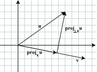
Summary of Section 3.6
In this section, we studied the following important concepts and ideas:
The component form of a vector v is written as v=⟨v1,v2⟩ and thei,j form of the same vector is v=v1i+v2j. Using this notation, we have
- The magnitude (or length) of the vector v is v=√v21+v22.
- The direction angle of v is θ, where 0∘≤θ<360∘, and cos(θ)=v1|v| and sin(θ)=v2|v|
- The horizontal and component and vertical component of the vector v and direction angle θ are v1=|v|cos(θ) and v2=|v|sin(θ)
For two vectors v and w with v=⟨v1,v2⟩=v1i+v2j and w=⟨w1,w2⟩=w1i+w2j and a scalar c:
- v+w=⟨v1+w1,v2+w2⟩=(v1+w1)i+(v2+w2)j
- v−w=⟨v1−w1,v2−w2⟩=(v1−w1)i+(v2−w2)j
- cv=⟨cv1,cv2⟩=(cv1)i+(cv2)j
- The dot product of v and w is u⋅v=u1v1+u2v2.
- If θ is the angle between v and w, then u⋅u=|u||v|cos(θ) or cos(θ)=u⋅v|u||v|
- The projection of the vector v onto the vector w projwv, is given by
projwv=v⋅w|w|2w=v⋅ww⋅ww
The projection of v orthogonal to w, denoted proj⊥wv, is
proj⊥wv=v−projwvWe note that w=proj⊥wv+projwv See Figure 3.6.7.
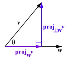
Figure 3.6.7: The Projection of v onto w