2.2: Solution by Graphing

Last updated
Save as PDF

Page ID: 40900

$ \newcommand{\vecs}[1]{\overset { \scriptstyle \rightharpoonup} {\mathbf{#1}} } $ $ \newcommand{\vecd}[1]{\overset{-\!-\!\rightharpoonup}{\vphantom{a}\smash {#1}}} $$\newcommand{\id}{\mathrm{id}}$ $ \newcommand{\Span}{\mathrm{span}}$ $ \newcommand{\kernel}{\mathrm{null}\,}$ $ \newcommand{\range}{\mathrm{range}\,}$ $ \newcommand{\RealPart}{\mathrm{Re}}$ $ \newcommand{\ImaginaryPart}{\mathrm{Im}}$ $ \newcommand{\Argument}{\mathrm{Arg}}$ $ \newcommand{\norm}[1]{\| #1 \|}$ $ \newcommand{\inner}[2]{\langle #1, #2 \rangle}$ $ \newcommand{\Span}{\mathrm{span}}$ $\newcommand{\id}{\mathrm{id}}$ $ \newcommand{\Span}{\mathrm{span}}$ $ \newcommand{\kernel}{\mathrm{null}\,}$ $ \newcommand{\range}{\mathrm{range}\,}$ $ \newcommand{\RealPart}{\mathrm{Re}}$ $ \newcommand{\ImaginaryPart}{\mathrm{Im}}$ $ \newcommand{\Argument}{\mathrm{Arg}}$ $ \newcommand{\norm}[1]{\| #1 \|}$ $ \newcommand{\inner}[2]{\langle #1, #2 \rangle}$ $ \newcommand{\Span}{\mathrm{span}}$$\newcommand{\AA}{\unicode[.8,0]{x212B}}$

In previous courses the solution of linear equations is covered, generally by separating the variables and constants on opposite sides of the equation to isolate the variable. In the previous chapter we examined the solution of quadratic equations, in which the variable is isolated using the technique of completing the square. The major difference between these methods of solution is that, in the solving of quadratic equations, we must contend with several different powers of the variable which makes it considerably more difficult to isolate the variable. There are formulas like the quadratic formula available to solve cubic $\left(x^{3}\right)$ and quartic $\left(x^{4}\right)$ equations, however these formulas are somewhat cumbersome and archaic. The primary method for solving eqautions of degree higher than 2 is solution by graphing or by algorithm.

Solution by algorithm is a very interesting process as there are many different algorithms available. Which algorithm is most appropriate often depends on the types of equations being solved and the technology available to solve them. Two major types of algorithms that rely on the graphincal representation of an equation are called "Double False Position" and "The Newton-Raphson Method." Many commonly available pieces of techonolgy use one of these methods. since we have graphing calculators available to us, we will focus on solution by graphing.

Whether using a TI (Texas Instruments) or Casio graphing calculator, or a software based graphing ustility such as Graph or Desmos, the solution of these equations focuses on finding the $x$ -intercepts of the graph since this is where the $y$ value is 0. The specific processes for solving equations using each of these different tools will be covered in class.
Example
Solve for $x$
$x^{3}-3 x^{2}=2 x-7$
The first step is to move all terms to one side of the equation and set them equal to zero.
$x^{3}-3 x^{2}-2 x+7=0$

Then we graph the function and look for which $x$ values will make the $y$ value equal to 0
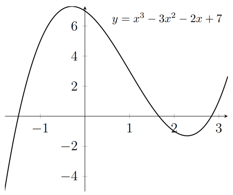
$clipboard_e33fa1feef9e5c0bb076eb8723f099773.png$
In this graph, we can see three roots, or $x$ -intercepts, where the graph crosses the $x$ -axis. These are the $x$ -values that make the $y$ -value equal to $0 .$ We can use the available technology to find these $x$ -values.
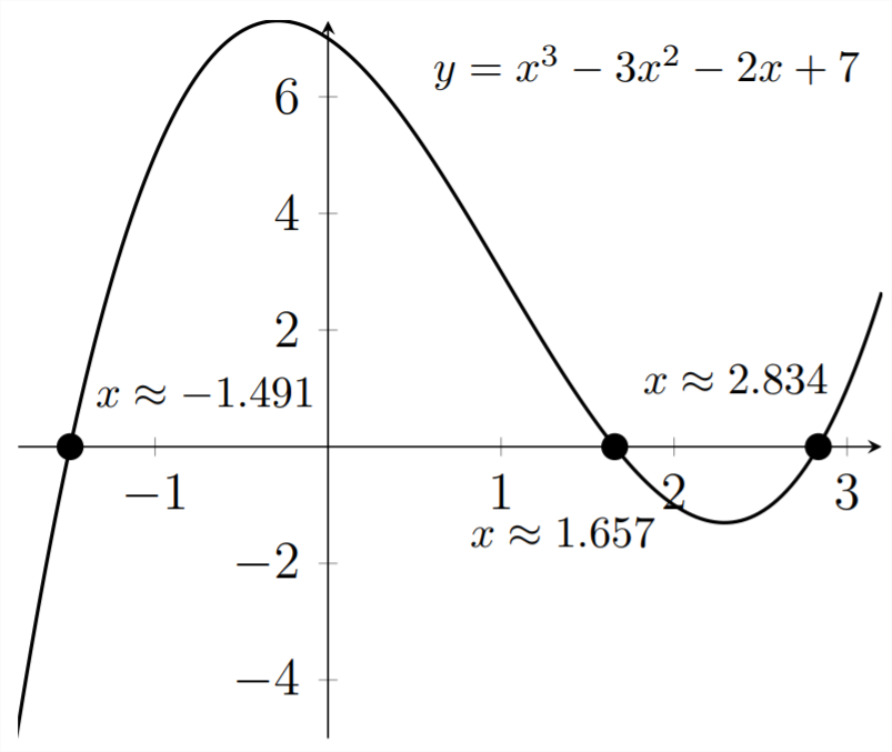
$clipboard_ec536203a344e401ed59a4b80b17e9690.png$
So, we can see that the solutions to the eqaution $x^{3}-3 x^{2}-2 x+7=0$ are $x \approx-1.491,1.657,2.834.$
We can check these answers by plugging them back into the original equation.

\[
\begin{aligned}
(-1.491)^{3}-3 *(-1.491)^{2}-2 *(-1.491)+7 &=-3.3146-3 * 2.223+2.982+7 \\
&=-3.3146-6.669+2.982+7 \\
&=-0.0016
\end{aligned}
\]
The result is not exactly 0 since our answers have been rounded off to the 1000 th place. If we wanted greater accuracy, then we should include greater accuracy in the value of our answers.
\[
\begin{aligned}
(1.657)^{3}-3 *(1.657)^{2}-2 *(1.657)+7 &=4.5495-3 * 2.7456-3.314+7 \\
&=4.5495-8.2368-3.314+7 \\
&=-0.0013
\end{aligned}
\]
and
\[
\begin{aligned}
(2.834)^{3}-3 *(2.834)^{2}-2 *(2.834)+7 &=22.7614-3 * 8.03155-5.668+7 \\
&=22.7614-24.09465-5.668+7 \\
&=-0.00125
\end{aligned}
\]

Exercises 2.2
Solve for $x$
1) $\quad 3 x^{3}-7 x^{2}-x+1=0$
2) $\quad 24 x^{4}+5 x^{2}-13 x+3=0$
3) $\quad 2 x^{3}-2 x^{2}-28 x+51=0$
4) $\quad 2 x^{3}+5 x^{2}-15 x+7=0$
5) $\quad x^{4}-4 x^{3}+x^{2}+6 x+1=0$
6) $\quad x^{4}+2 x^{3}+x^{2}-x-6=0$
7) $\quad x^{4}-5 x^{3}-3 x^{2}+17 x-9=0$
8) $\quad 2 x^{3}-5 x-3=0$
9) $\quad x^{4}-4 x^{3}-7 x^{2}-36 x-18=0$
10) $\quad 6 x^{3}-25 x^{2}+21 x+10=0$
11) $\quad 2 x^{4}-5 x^{3}+x^{2}+4 x-2=0$
12) $\quad x^{4}+x^{3}-5 x^{2}+x-4=0$