6.2: Zeros of Polynomials

In the previous section we studied the end-behavior of polynomials. We know that a polynomial’s end-behavior is identical to the end-behavior of its leading term. Our focus was concentrated on the far right- and left-ends of the graph and not upon what happens in-between. In this section, our focus shifts to the interior. There are two important areas of concentration: the local maxima and minima of the polynomial, and the location of the x-intercepts or zeros of the polynomial. In this section we concentrate on finding the zeros of the polynomial.

Zeros

Let’s begin with a formal definition of the zeros of a polynomial.

Definition: Zero of the Polynomial

Let \(p(x)=a_{0}+a_{1} x+a_{2} x^{2}+\cdots+a_{n} x^{n}\) be a polynomial with real coefficients. We say that \(a\) is a zero of the polynomial if and only if \(p(a) = 0\).

The definition also holds if the coefficients are complex, but that’s a topic for a more advanced course.

For example, −5 is a zero of the polynomial \(p(x)=x^{2}+3 x-10\) because

\[\begin{aligned} p(-5) &=(-5)^{2}+3(-5)-10 \\ &=25-15-10 \\ &=0 \end{aligned} \nonumber \]

Similarly, −1 is a zero of the polynomial \(p(x)=x^{3}+3 x^{2}-x-3\) because

\[\begin{aligned} p(-1) &=(-1)^{3}+3(-1)^{2}-(-1)-3 \\ &=-1+3+1-3 \\ &=0 \end{aligned} \nonumber \]

Let’s look at a more extensive example.

Example \(\PageIndex{1}\)

Find the zeros of the polynomial defined by

\[p(x)=(x+3)(x-2)(x-5). \nonumber \]

Solution

At first glance, the function does not appear to have the form of a polynomial. However, two applications of the distributive property provide the product of the last two factors.

\[\begin{aligned} p(x) &=(x+3)(x(x-5)-2(x-5)) \\ &=(x+3)\left(x^{2}-5 x-2 x+10\right) \\ &=(x+3)\left(x^{2}-7 x+10\right) \end{aligned} \nonumber \]

A third and fourth application of the distributive property reveals the nature of our function.

\[\begin{aligned} p(x) &=x\left(x^{2}-7 x+10\right)+3\left(x^{2}-7 x+10\right) \\ &=x^{3}-7 x^{2}+10 x+3 x^{2}-21 x+30 \\ &=x^{3}-4 x^{2}-11 x+30 \end{aligned} \nonumber \]

Hence, p is clearly a polynomial. However, the original factored form provides quicker access to the zeros of this polynomial. Using Definition 1, we need to find values of x that make p(x) = 0. That is, we need to solve the equation \[p(x)=0 \nonumber \]

Of course, p(x) = (x + 3)(x − 2)(x − 5), so, equivalently, we need to solve the equation

\[(x+3)(x-2)(x-5)=0 \nonumber \]

By the zero product property, either

\[x+3=0 \quad \text { or } \quad x-2=0 \quad \text { or } \quad x-5=0 \nonumber \]

These are linear (first degree) equations, each of which can be solved independently. Thus, either

\[x=-3 \quad \text { or } \quad x=2 \quad \text { or } \quad x=5 \nonumber \]

Hence, the zeros of the polynomial p are −3, 2, and 5.

Let’s use equation (4) to check that −3 is a zero of the polynomial p. Substitute −3 for x in \(p(x)=x^{3}-4 x^{2}-11 x+30\).

\[\begin{aligned} p(-3) &=(-3)^{3}-4(-3)^{2}-11(-3)+30 \\ &=-27-36+33+30 \\ &=0 \end{aligned} \nonumber \]

This calculation verifies that −3 is a zero of the polynomial p. However, it is much easier to check that −3 is a zero of the polynomial using equation (3). Substitute −3 for x in p(x) = (x + 3)(x − 2)(x − 5).

\[\begin{aligned} p(-3) &=(-3+3)(-3-2)(-3-5) \\ &=(0)(-5)(-8) \\ &=0 \end{aligned} \nonumber \]

We’ll leave it to our readers to check that 2 and 5 are also zeros of the polynomial p.

It’s very important to note that once you know the linear (first degree) factors of a polynomial, the zeros follow with ease. In the last example, p(x) = (x+3)(x−2)(x−5), so the linear factors are x + 3, x − 2, and x − 5. Consequently, the zeros are −3, 2, and 5.

Before continuing, we take a moment to review an important multiplication pattern.

The Difference of Two Squares

A special multiplication pattern that appears frequently in this text is called the difference of two squares. Use the distributive property to expand (a + b)(a − b).

\[\begin{aligned}(a+b)(a-b) &=a(a-b)+b(a-b) \\ &=a^{2}-a b+b a-b^{2} \end{aligned} \nonumber \]

Since \(ab = ba\), we have the following result.

Property 5: The Difference of Two Squares Pattern

\[(a+b)(a-b)=a^{2}-b^{2} \nonumber \]

Thus, if you have two binomials with identical first and second terms, but the terms of one are separated by a plus sign, while the terms of the second are separated by a minus sign, then you multiply by squaring the first and second terms and separating these squares with a minus sign. Hence the name, the “difference of two squares.”

For example,

\[(2 x+3)(2 x-3)=(2 x)^{2}-(3)^{2}=4 x^{2}-9 \nonumber \]

Note how we simply squared the matching first and second terms and then separated our squares with a minus sign. In similar fashion,

\[\begin{aligned}(x+5)(x-5) &=x^{2}-25 \\(5 x+4)(5 x-4) &=25 x^{2}-16 \\(3 x-7)(3 x+7) &=9 x^{2}-49 \end{aligned} \nonumber \]

In each case, note how we squared the matching first and second terms, then separated the squares with a minus sign.

Once you’ve mastered multiplication using the “Difference of Squares” pattern, it is easy to factor using the same pattern. You simply reverse the procedure. For example

\[4 x^{2}-9=(2 x+3)(2 x-3) \nonumber \]

We start by taking the square root of the two squares. Thus, the square root of 4\(x^{2}\) is 2x and the square root of 9 is 3. We then form two binomials with the results 2x and 3 as matching first and second terms, separating one pair with a plus sign, the other pair with a minus sign.

In similar fashion, \[9 x^{2}-49=(3 x+7)(3 x-7) \nonumber \]

Again, note how we take the square root of each term, form two binomials with the results, then separate one pair with a plus, the other with a minus.

We’ll find the “Difference of Squares” pattern handy in what follows.

Finding Zeros by Factoring

We will now explore how we can find the zeros of a polynomial by factoring, followed by the application of the zero product property. It is important to understand that the polynomials of this section have been carefully selected so that you will be able to factor them using the various techniques that follow.

Let’s explore factoring by grouping.

Example \(\PageIndex{2}\)

Find the zeros of the polynomial \[p(x)=x^{3}+2 x^{2}-25 x-50 \nonumber \]

Solution

In Example \(\PageIndex{1}\) we learned that it is easy to spot the zeros of a polynomial if the polynomial is expressed as a product of linear (first degree) factors. In this example, the polynomial is not factored, so it would appear that the first thing we’ll have to do is factor our polynomial.

Whenever you are presented with a four term expression, one thing you can try is factoring by grouping. So, with this thought in mind, let’s factor an x out of the first two terms, then a −25 out of the second two terms.

\[\begin{aligned} p(x) &=x^{3}+2 x^{2}-25 x-50 \\ &=x^{2}(x+2)-25(x+2) \end{aligned} \nonumber \]

Note that this last result is the difference of two terms. The polynomial is not yet fully factored as it is not yet a product of two or more factors. However, note that each of the two terms has a common factor of x + 2. Let’s factor out this common factor.

\[p(x)=\left(x^{2}-25\right)(x+2) \nonumber \]

We’ve still not completely factored our polynomial. The first factor is the difference of two squares and can be factored further.

\[p(x)=(x+5)(x-5)(x+2) \nonumber \]

The polynomial p is now fully factored. To find the zeros of the polynomial p, we need to solve the equation \[p(x)=0 \nonumber \]

However, p(x) = (x + 5)(x − 5)(x + 2), so equivalently, we need to solve the equation \[(x+5)(x-5)(x+2)=0 \nonumber \]

We can use the zero product property. Either \[x+5=0 \quad \text { or } \quad x-5=0 \quad \text { or } \quad x+2=0 \nonumber \]

Again, each of these linear (first degree) equations can be solved independently. Either \[x=-5 \quad \text { or } \quad x=5 \quad \text { or } \quad x=-2 \nonumber \]

Thus, the zeros of the polynomial p are −5, 5, and −2. We’ll leave it to our readers to check these results.

Again, it is very important to realize that once the linear (first degree) factors are determined, the zeros of the polynomial follow. In this example, the linear factors are x + 5, x − 5, and x + 2. It immediately follows that the zeros of the polynomial are −5, 5, and −2.

In the next example, we will see that sometimes the first step is to factor out the greatest common factor.

Example \(\PageIndex{3}\)

Find the zeros of the polynomial \[p(x)=x^{4}+2 x^{3}-16 x^{2}-32 x \nonumber \]

Solution

To find the zeros of the polynomial, we need to solve the equation \[p(x)=0 \nonumber \]

Equivalently, because \(p(x)=x^{4}+2 x^{3}-16 x^{2}-32 x\), we need to solve the equation

\[x^{4}+2 x^{3}-16 x^{2}-32 x=0 \nonumber \]

Note that each term on the left-hand side has a common factor of x. Thus, our first step is to factor out this common factor of x.

\[x\left[x^{3}+2 x^{2}-16 x-32\right]=0 \nonumber \]

The four-term expression inside the brackets looks familiar. Let’s try factoring by grouping. Factor an \(x^2\) out of the first two terms, then a −16 from the third and fourth terms.

\[x\left[x^{2}(x+2)-16(x+2)\right]=0 \nonumber \]

We now have a common factor of x + 2, so we factor it out.

\[x\left[\left(x^{2}-16\right)(x+2)\right]=0 \nonumber \]

The brackets are no longer needed (multiplication is associative) so we leave them off, then use the difference of squares pattern to factor \(x^2 − 16\).

\[x(x+4)(x-4)(x+2)=0 \nonumber \]

The zero product property tells us that either

\[x=0 \quad \text { or } \quad \text { or } \quad x+4=0 \quad \text { or } \quad x-4=0 \quad \text { or } \quad \text { or } \quad x+2=0 \nonumber \]

Each of these linear (first degree) factors can be solved independently. Either

\[x=0 \quad \text { or } \quad x=-4 \quad \text { or } \quad x=4 \quad \text { or } \quad x=-2 \nonumber \]

Thus, the zeros of the polynomial p are 0, −4, 4, and −2. We’ll leave it to our readers to check these results.

Again, it is very important to note that once you’ve determined the linear (first degree) factors of a polynomial, then you know the zeros. In this case, the linear factors are x, x + 4, x − 4, and x + 2. Therefore, the zeros are 0, −4, 4, and −2, respectively. This discussion leads to a result called the Factor Theorem.

Factor Theorem

Let \(p(x)=a_{0}+a_{1} x+a_{2} x^{2}+\ldots+a_{n} x^{n}\) be a polynomial with real coefficients. If x − a is a factor of the polynomial p(x), then a is a zero of the polynomial. That is, if x − a is a factor of the polynomial p(x), then p(a) = 0.

The upshot of all of these remarks is the fact that, if you know the linear factors of the polynomial, then you know the zeros. The converse is also true, but we will not need it in this course.

Let’s examine the connection between the zeros of the polynomial and the x-intercepts of the graph of the polynomial.

The x-intercepts and the Zeros of a Polynomial

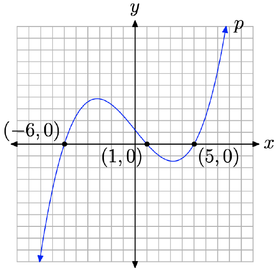
For the discussion that follows, let’s assume that the independent variable is x and the dependent variable is y. Corresponding to these assignments, we will also assume that we’ve labeled the horizontal axis with x and the vertical axis with y, as shown in Figure \(\PageIndex{1}\).

The key fact for the remainder of this section is that a function is zero at the points where its graph crosses the x-axis. The phrases “function values” and “y-values” are equivalent (provided your dependent variable is y), so when you are asked where your function value is equal to zero, you are actually being asked “where is your y-value equal to zero?” Of course, y = 0 where the graph of the function crosses the horizontal axis (again, providing you are using the letter y for your dependent variable—labeling the vertical axis with y).

A polynomial is a function, so, like any function, a polynomial is zero where its graph crosses the horizontal axis. As you can see in Figure \(\PageIndex{1}\), the graph of the polynomial crosses the horizontal axis at x = −6, x = 1, and x = 5. Note that at each of these intercepts, the y-value (function value) equals zero. The zeros of the polynomial are −6, 1, and 5. Therefore the x-intercepts of the graph of the polynomial are located at (−6, 0), (1, 0), and (5, 0).

Figure \(\PageIndex{1}\). A function is zero where its graph crosses the horizontal axis.

Let’s use these ideas to plot the graphs of several polynomials.

Example \(\PageIndex{4}\)

Sketch the graph of the polynomial in Example \(\PageIndex{2}\).

Solution

In Example \(\PageIndex{2}\), the polynomial \(p(x)=x^{3}+2 x^{2}-25 x-50\) factored into linear factors \[p(x)=(x+5)(x-5)(x+2) \nonumber \]

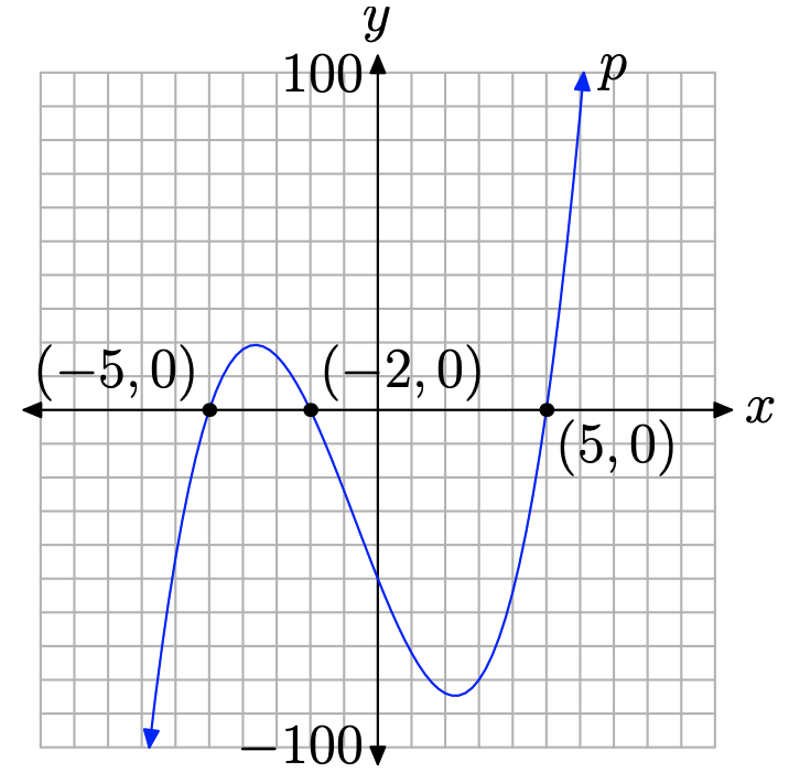
Consequently, the zeros of the polynomial were −5, 5, and −2. Thus, the x-intercepts of the graph of the polynomial are located at (−5, 0), (5, 0), and (−2, 0).

The polynomial \(p(x)=x^{3}+2 x^{2}-25 x-50\) has leading term \(x^3\). Consequently, as we swing our eyes from left to right, the graph of the polynomial p must rise from negative infinity, wiggle through its x-intercepts, then continue to rise to positive infinity. We have no choice but to sketch a graph similar to that in Figure \(\PageIndex{2}\).

Note that there are two “turning points” of the polynomial in Figure \(\PageIndex{2}\). You might ask how we knew where to put these “turning points” of the polynomial. The answer is “we didn’t know where to put them.” We know they have to be there, but we don’t know their precise location. That’s why we haven’t scaled the vertical axis, because without the aid of a calculator, it’s hard to determine the precise location of the turning points shown in Figure \(\PageIndex{2}\).

However, note that knowledge of the end-behavior and the zeros of the polynomial allows us to construct a reasonable facsimile of the actual graph. If we want more accuracy than a rough approximation provides, such as the accuracy displayed in Figure \(\PageIndex{2}\), we’ll have to use our graphing calculator, as demonstrated in Figure \(\PageIndex{3}\).

Figure \(\PageIndex{2}\). The graph rises from negative infinity, wiggles through its x-intercepts, then rises to positive infinity.

Figure \(\PageIndex{3}\). The graph of \(p(x)=x^{3}+2 x^{2}-25 x-50\) and the window settings used.

We’ll have more to say about the “turning points” (relative extrema) in the next section. For now, let’s continue to focus on the end-behavior and the zeros.

Let’s look at another example.

Example \(\PageIndex{5}\)

Sketch the graph of the polynomial in Example \(\PageIndex{3}\).

Solution

In Example \(\PageIndex{3}\), the polynomial \(p(x)=x^{4}+2 x^{3}-16 x^{2}-32 x\) factored into a product of linear factors

\[p(x)=x(x+4)(x-4)(x+2) \nonumber \]

Consequently, the zeros of the polynomial are 0, −4, 4, and −2. Thus, the x-intercepts of the graph of the polynomial are located at (0, 0), (−4, 0), (4, 0) and (−2, 0).

The polynomial \(p(x)=x^{4}+2 x^{3}-16 x^{2}-32 x\) has leading term \(x^4\). Consequently, as we swing our eyes from left to right, the graph of the polynomial p must fall from positive infinity, wiggle through its x-intercepts, then rise back to positive infinity. We have no choice but to sketch a graph similar to that in Figure \(\PageIndex{4}\).

Figure \(\PageIndex{4}\). The graph falls from positive infinity, wiggles through its x-intercepts, then rises back to positive infinity.

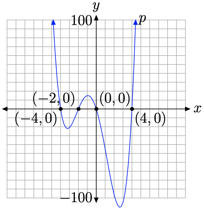
Again, we can draw a sketch of the graph without the use of the calculator, using only the end-behavior and zeros of the polynomial. However, if we want the accuracy depicted in Figure \(\PageIndex{4}\), particularly finding correct locations of the “turning points,” we’ll have to resort to the use of a graphing calculator. This is shown in Figure \(\PageIndex{5}\).

Figure \(\PageIndex{5}\). The graph of \(p(x)=x^{4}-20 x^{2}+64\) and the window settings used.

Let’s look at a final example that requires factoring out a greatest common factor followed by the ac-test.

Example \(\PageIndex{6}\)

Find the zeros of the polynomial \[p(x)=4 x^{3}-2 x^{2}-30 x \nonumber \]

Solution

First, notice that each term of this trinomial is divisible by 2x. This is the greatest common divisor, or equivalently, the greatest common factor. You should always look to factor out the greatest common factor in your first step.

\[\begin{aligned} p(x) &=4 x^{3}-2 x^{2}-30 x \\ &=2 x\left[2 x^{2}-x-15\right] \end{aligned} \nonumber \]

Next, compare the trinomial \(2 x^{2}-x-15\) with \(a x^{2}+b x+c\) and note that ac = −30. The integer pair {5, −6} has product −30 and sum −1. Rewrite the middle term of \(2 x^{2}-x-15\) in terms of this pair and factor by grouping.

\[\begin{aligned} p(x) &=2 x\left[2 x^{2}+5 x-6 x-15\right] \\ &=2 x[x(2 x+5)-3(2 x+5)] \\ &=2 x(x-3)(2 x+5) \end{aligned} \nonumber \]

To find the zeros, we need to solve the polynomial equation p(x) = 0, or equivalently,

\[2 x(x-3)(2 x+5)=0 \nonumber \]

Using the zero product property, either

\[2 x=0, \quad \text { or } \quad x-3=0, \quad \text { or } \quad 2 x+5=0 \nonumber \]

Each of these linear factors can be solved independently. Thus, either

\[x=0, \quad \text { or } \quad x=3, \quad \text { or } \quad x=-\frac{5}{2} \nonumber \]

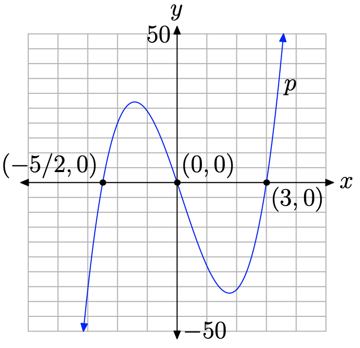
Thus, the zeros of the polynomial are 0, 3, and −5/2.

Alternatively, one can factor out a 2 from the third factor in equation (12).

\[\begin{aligned} p(x) &=2 x(x-3)(2)\left(x+\frac{5}{2}\right) \\ &=4 x(x-3)\left(x+\frac{5}{2}\right) \end{aligned} \nonumber \]

In this form,

• x is a factor, so x = 0 is a zero,
• x − 3 is a factor, so x = 3 is a zero, and
• x + 5/2 is a factor, so x = −5/2 is a zero.

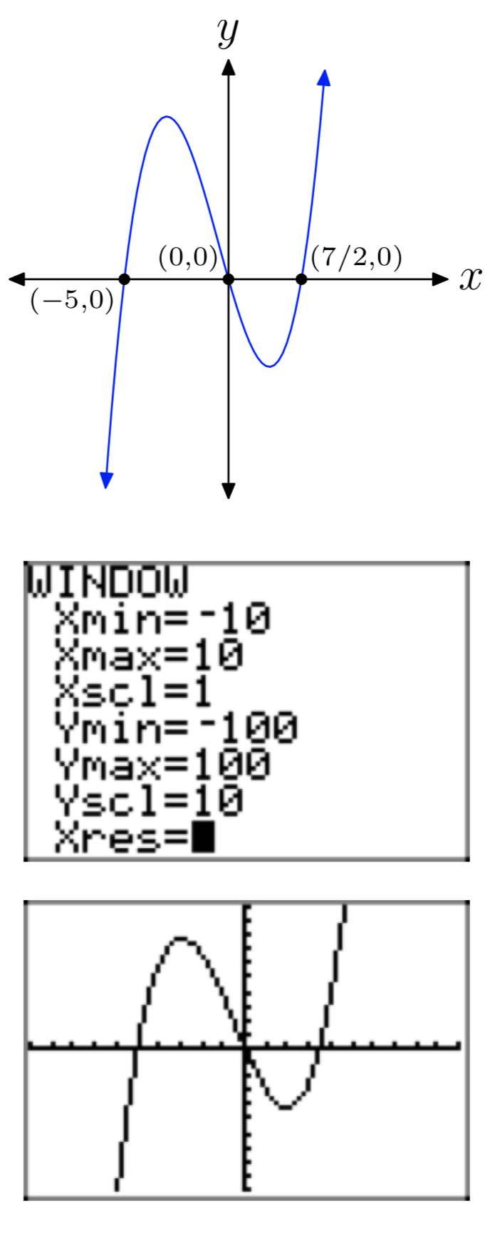
The leading term of \(p(x)=4 x^{3}-2 x^{2}-30 x\) is 4\(x^{2}\), so as our eyes swing from left to right, the graph of the polynomial must rise from negative infinity, wiggle through its zeros, then rise to positive infinity. The graph must therefore be similar to that shown in Figure \(\PageIndex{6}\).

Again, the intercepts and end-behavior provide ample clues to the shape of the graph, but, if we want the accuracy portrayed in Figure 6, then we must rely on the graphing calculator. The graph and window settings used are shown in Figure \(\PageIndex{7}\).

Figure \(\PageIndex{6}\). The graph rises from negative infinity, wiggles through its zeros, then rises to positive infinity

Figure \(\PageIndex{7}\). The graph of \(p(x)=4 x^{3}-2 x^{2}-30 x\) and the window settings used.

Exercise

In Exercises 1-6, use direct substitution to show that the given value is a zero of the given polynomial.

Exercise \(\PageIndex{1}\)

\(p(x) = x^3−3x^2−13x+15\), x = −3

Answer

p(−3) = (−3)3−3(−3)2−13(−3)+15 = 0

Exercise \(\PageIndex{2}\)

\(p(x) = x^3−2x^2−13x−10\), x = −2

Exercise \(\PageIndex{3}\)

\(p(x) = x^4−x^3−12x^2\), x = 4

Answer

\(p(4) = 4^4−4^3−12(4)^2 = 0\)

Exercise \(\PageIndex{4}\)

\(p(x) = x^4−2x^3−3x^2\), x = −1

Exercise \(\PageIndex{5}\)

\(p(x) = x^4+x^2−20\), x = −2

Answer

\(p(−2) = (−2)^4+(−2)^2−20 = 0\)

Exercise \(\PageIndex{6}\)

\(p(x) = x^4+x^3−19x^2+11x+30\), x = −1

In Exercises 7-28, identify all of the zeros of the given polynomial without the aid of a calculator. Use an algebraic technique and show all work (factor when necessary) needed to obtain the zeros.

Exercise \(\PageIndex{7}\)

p(x) = (x−2)(x+4)(x−5)

Answer

−4, 2, and 5

Exercise \(\PageIndex{8}\)

p(x) = (x−1)(x−3)(x+8)

Exercise \(\PageIndex{9}\)

p(x) = −2(x−3)(x+4)(x−2)

Answer

−4, 2, and 3

Exercise \(\PageIndex{10}\)

p(x) = −3(x+1)(x−1)(x−8)

Exercise \(\PageIndex{11}\)

p(x) = x(x−3)(2x+1)

Answer

\(−\frac{1}{2}\), 0, and 3

Exercise \(\PageIndex{12}\)

p(x) = −3x(x+5)(3x−2)

Exercise \(\PageIndex{13}\)

p(x) = −2(x+3)(3x−5)(2x+1)

Answer

−3, \(−\frac{1}{2}\), and \(\frac{5}{3}\)

Exercise \(\PageIndex{14}\)

p(x) = 3(x−2)(2x+5)(3x−4)

Exercise \(\PageIndex{15}\)

\(p(x) = 3x^3+5x^2−12x−20\)

Answer

−2, \(−\frac{5}{3}\), and 2

Exercise \(\PageIndex{16}\)

\(p(x) = 3x^3+x^2−12x−4\)

Exercise \(\PageIndex{17}\)

\(p(x) = 2x^3+5x^2−2x−5\)

Answer

\(−\frac{5}{2}\), −1, and 1

Exercise \(\PageIndex{18}\)

\(p(x) = 2x^3−5x^2−18x+45\)

Exercise \(\PageIndex{19}\)

\(p(x) = x^4+4x^3−9x^2−36x\)

Answer

0, −3, 3, and −4

Exercise \(\PageIndex{20}\)

\(p(x) = −x^4+4x^3+x^2−4x\)

Exercise \(\PageIndex{21}\)

\(p(x) = −2x^4−10x^3+8x^2+40x\)

Answer

0, −2, 2, and −5

Exercise \(\PageIndex{22}\)

\(p(x) = 3x^4+6x^3−75x^2−150x\)

Exercise \(\PageIndex{23}\)

\(p(x) = 2x^3−7x^2−15x\)

Answer

\(−\frac{3}{2}\), 0, and 5

Exercise \(\PageIndex{24}\)

\(p(x) = 2x^3−x^2−10x\)

Exercise \(\PageIndex{25}\)

\(p(x) = −6x^3+4x^2+16x\)

Answer

\(−\frac{4}{3}\), 0, and 2

Exercise \(\PageIndex{26}\)

\(p(x) = 9x^3+3x^2−30x\)

Exercise \(\PageIndex{27}\)

\(p(x) = −2x^7−10x^6+8x^5+40x^4\)

Answer

0, −2, 2, and −5

Exercise \(\PageIndex{28}\)

\(p(x) = 6x^5−21x^4−45x^3\)

In Exercises 29-34, the graph of a polynomial is given. Perform each of the following tasks

1. Copy the image onto your homework paper. Label and scale your axes, then label each x-intercept with its coordinates.
2. Identify the zeros of the polynomial.

Exercise \(\PageIndex{29}\)

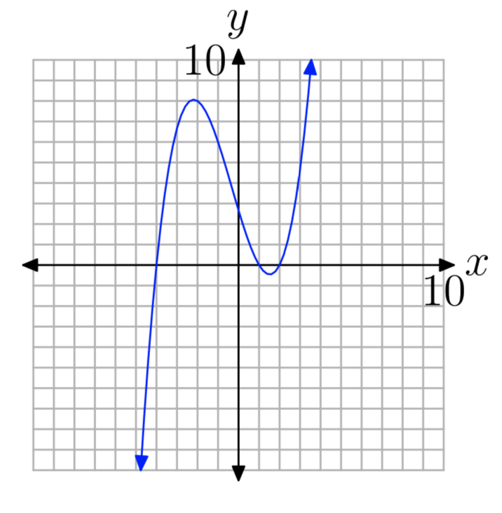
Answer

Zeros: −4, 1, and 2

Exercise \(\PageIndex{30}\)

Exercise \(\PageIndex{31}\)

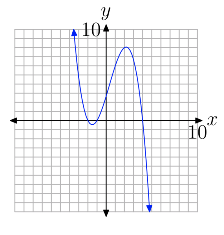
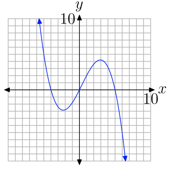
Answer

Zeros: −4, 0, and 5

Exercise \(\PageIndex{32}\)

Exercise \(\PageIndex{33}\)

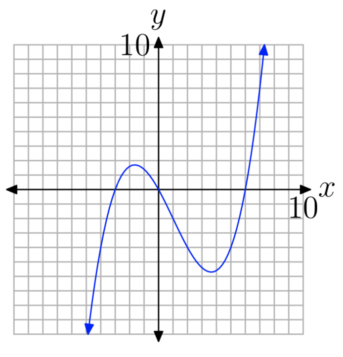
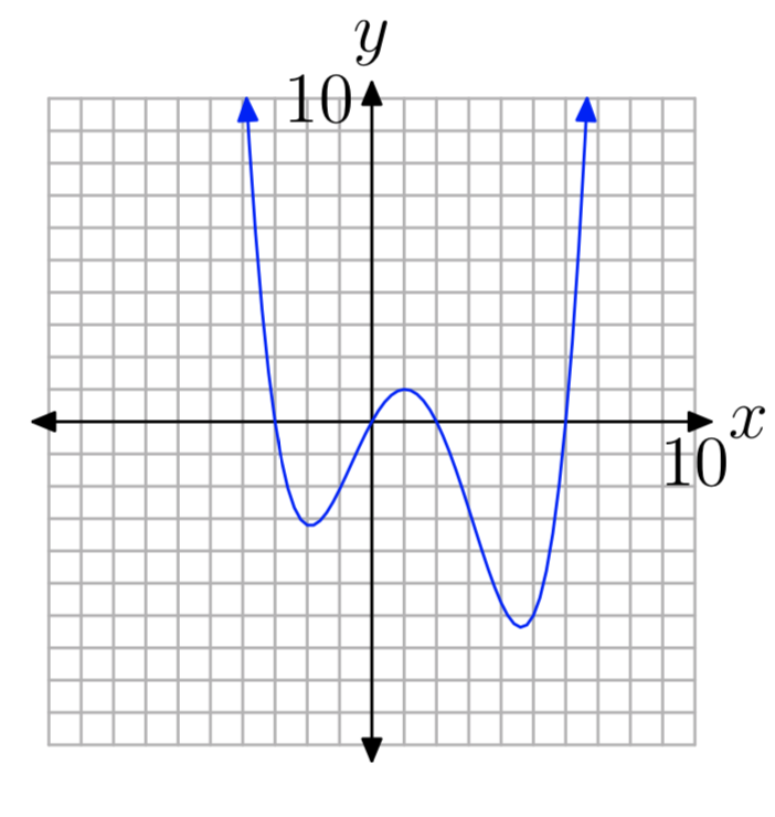
Answer

Zeros: 0, 6, −3, 2

Exercise \(\PageIndex{34}\)

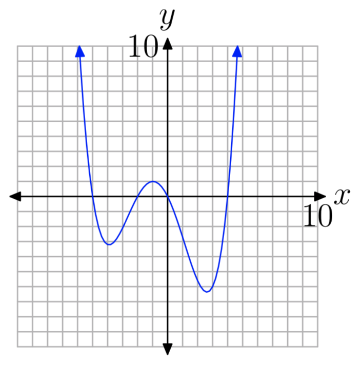
For each of the polynomials in Exercises 35-46, perform each of the following tasks.

1. Factor the polynomial to obtain the zeros. Show your work.
2. Set up a coordinate system on graph paper. Label and scale the horizontal axis. Use the zeros and end-behavior to help sketch the graph of the polynomial without the use of a calculator.
3. Verify your result with a graphing calculator.

Exercise \(\PageIndex{35}\)

\(p(x) = 5x^3+x^2−45x−9\)

Answer

Exercise \(\PageIndex{36}\)

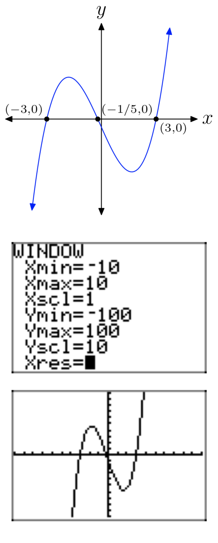
\(p(x) = 4x^3+3x^2−64x−48\)

Exercise \(\PageIndex{37}\)

\(p(x) = 4x^3−12x^2−9x+27\)

Answer

Exercise \(\PageIndex{38}\)

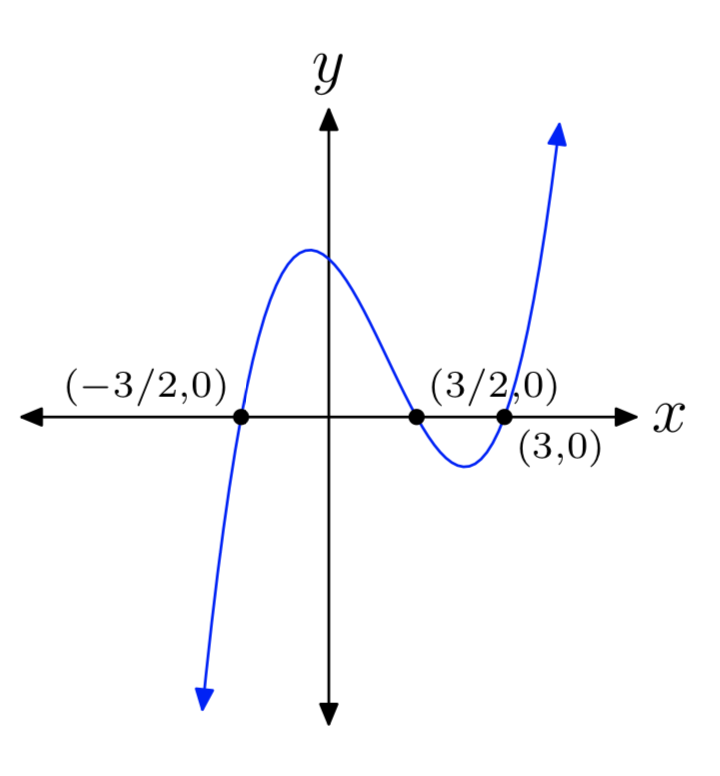
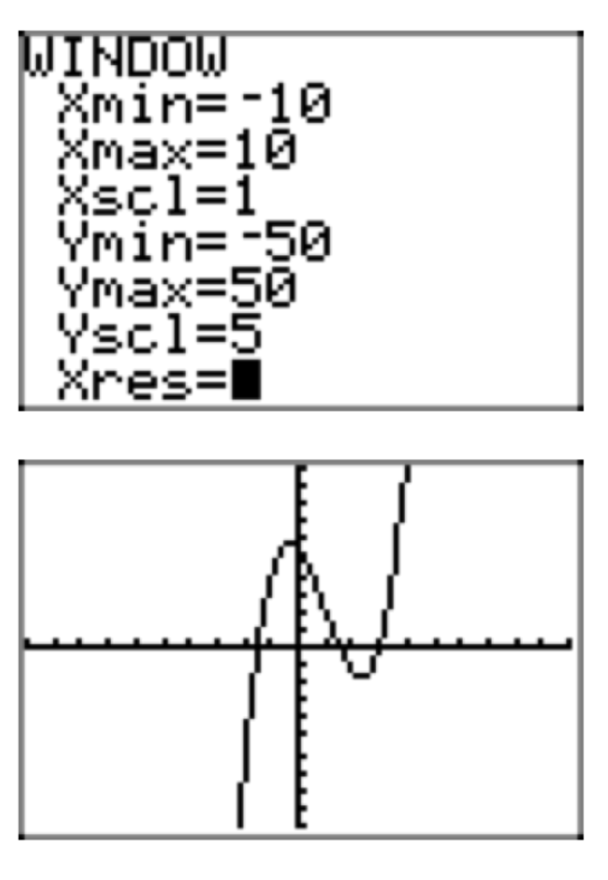
\(p(x) = x^3+x^2−16x−16\)

Exercise \(\PageIndex{39}\)

\(p(x) = x^4+2x^3−25x^2−50x\)

Answer

Exercise \(\PageIndex{40}\)

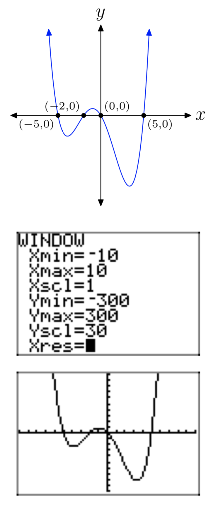
\(p(x) = −x^4−5x^3+4x^2+20x\)

Exercise \(\PageIndex{41}\)

\(p(x) = −3x^4−9x^3+3x^2+9x\)

Answer

Exercise \(\PageIndex{42}\)

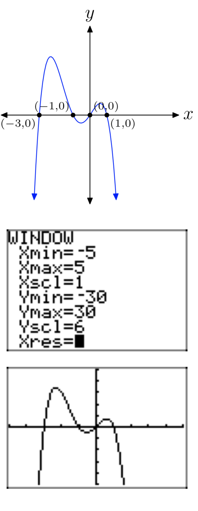
\(p(x) = 4x^4−29x^2+25\)

Exercise \(\PageIndex{43}\)

\(p(x) = −x^3−x^2+20x\)

Answer

Exercise \(\PageIndex{44}\)

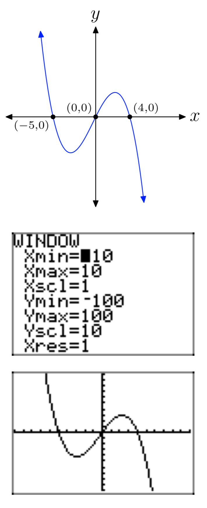
\(p(x) = 2x^3−7x^2−30x\)

Exercise \(\PageIndex{45}\)

\(p(x) = 2x^3+3x^2−35x\)

Answer

Exercise \(\PageIndex{46}\)

\(p(x) = −2x^3−11x^2+21x\)