3.7: The Gibbs Phenomenon

We have seen from the Gibbs Phenomenon when there is a jump discontinuity in the periodic extension of a function, whether the function originally had a discontinuity or developed one due to a mismatch in the values of the endpoints. This can be seen in Figures 3.3.6, 3.4.2 and 3.4.4. The Fourier series has a difficult time converging at the point of discontinuity and these graphs of the Fourier series show a distinct overshoot which does not go away. This is called the Gibbs phenomenon\(^{1}\) and the amount of overshoot can be computed.

In one of our first examples, Example 3.2.3, we found the Fourier series representation of the piecewise defined function \[f(x)=\left\{\begin{array}{cc} 1, & 0<x<\pi, \\ -1, & \pi<x<2 \pi, \end{array}\right.\label{eq:1}\] to be \[f(x) \sim \frac{4}{\pi} \sum_{k=1}^{\infty} \frac{\sin (2 k-1) x}{2 k-1}\label{eq:2} \]

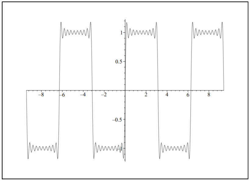
In Figure \(\PageIndex{1}\) we display the sum of the first ten terms. Note the wiggles, overshoots and under shoots. These are seen more when we plot the representation for \(x \in[-3 \pi, 3 \pi]\), as shown in Figure \(\PageIndex{2}\).

Figure \(\PageIndex{1}\): The Fourier series representation of a step function on \([-\pi, \pi]\) for \(N=10\).

Figure \(\PageIndex{2}\): The Fourier series representation of a step function on \([-\pi, \pi]\) for \(N=10\) plotted on \([-3 \pi, 3 \pi]\) displaying the periodicity.

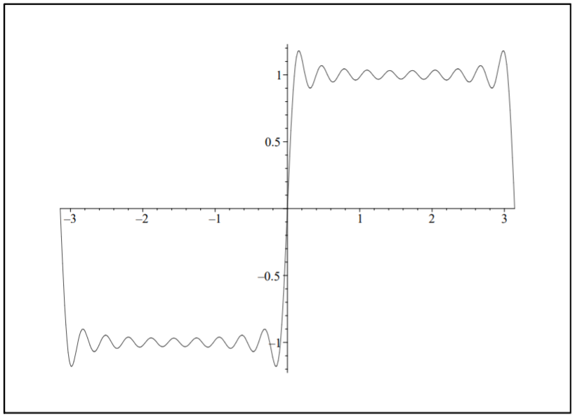
We note that the overshoots and undershoots occur at discontinuities in the periodic extension of \(f(x)\). These occur whenever \(f(x)\) has a discontinuity or if the values of \(f(x)\) at the endpoints of the domain do not agree.

Figure \(\PageIndex{3}\): The Fourier series representation of a step function on \([-\pi, \pi]\) for \(N=20\).

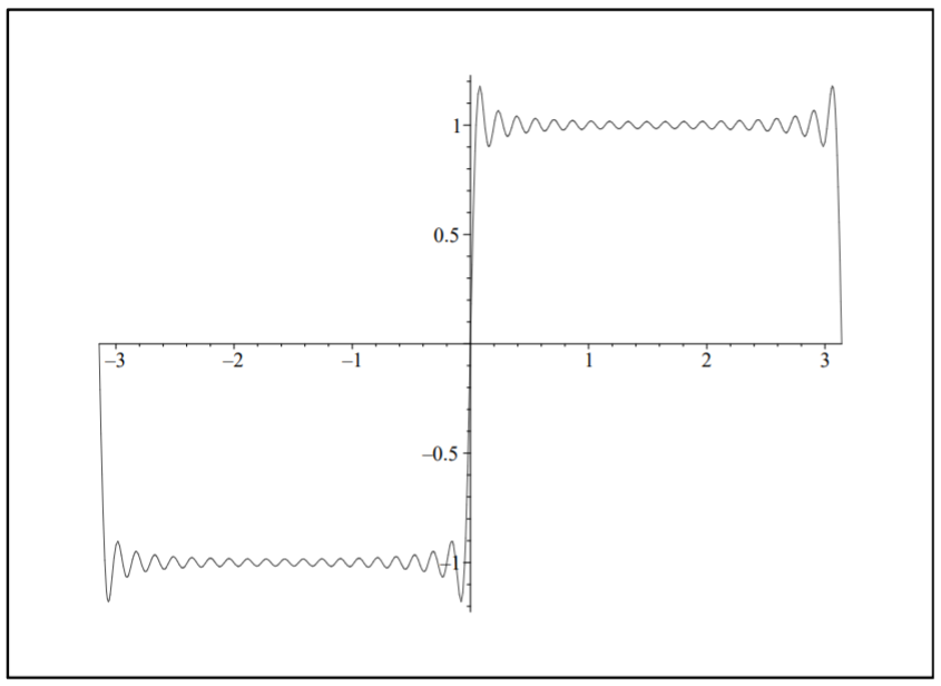
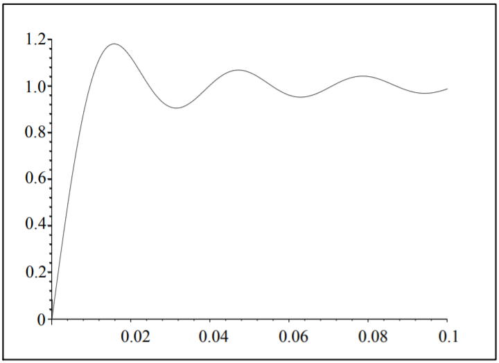
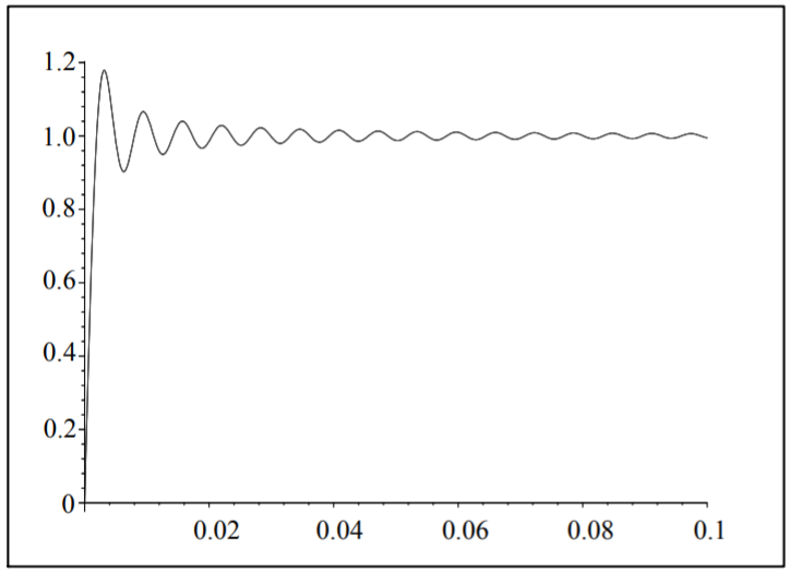
One might expect that we only need to add more terms. In Figure \(\PageIndex{3}\) we show the sum for twenty terms. Note the sum appears to converge better for points far from the discontinuities. But, the overshoots and undershoots are still present. In Figures \(\PageIndex{4}\) and \(\PageIndex{5}\) show magnified plots of the overshoot at \(x = 0\) for \(N = 100\) and \(N = 500\), respectively. We see that the overshoot persists. The peak is at about the same height, but its location seems to be getting closer to the origin. We will show how one can estimate the size of the overshoot.

Figure \(\PageIndex{4}\): The Fourier series representation of a step function on \([-\pi, \pi]\) for \(N=100\).

Figure \(\PageIndex{5}\): The Fourier series representation of a step function on \([-\pi, \pi]\) for \(N=500\).

We can study the Gibbs phenomenon by looking at the partial sums of general Fourier trigonometric series for functions \(f(x)\) defined on the interval \([-L, L]\). Writing out the partial sums, inserting the Fourier coefficients and rearranging, we have \[\begin{aligned}S_{N}(x)=&a_{0}+\sum_{n=1}^{N}\left[a_{n} \cos \frac{n \pi x}{L}+b_{n} \sin \frac{n \pi x}{L}\right] \\ =& \frac{1}{2 L} \int_{-L}^{L} f(y) d y+\sum_{n=1}^{N}\left[\left(\frac{1}{L} \int_{-L}^{L} f(y) \cos \frac{n \pi y}{L} d y\right) \cos \frac{n \pi x}{L}\right.\\ &\left.+\left(\frac{1}{L} \int_{-L}^{L} f(y) \sin \frac{n \pi y}{L} d y .\right) \sin \frac{n \pi x}{L}\right] \\ =& \frac{1}{L} \int_{-L}^{L}\left\{\frac{1}{2}\right.\\ &\left.+\sum_{n=1}^{N}\left(\cos \frac{n \pi y}{L} \cos \frac{n \pi x}{L}+\sin \frac{n \pi y}{L} \sin \frac{n \pi x}{L}\right)\right\} f(y) d y \\ =& \frac{1}{L} \int_{-L}^{L}\left\{\frac{1}{2}+\sum_{n=1}^{N} \cos \frac{n \pi(y-x)}{L}\right\} f(y) d y \\ \equiv & \frac{1}{L} \int_{-L}^{L} D_{N}(y-x) f(y) d y \end{aligned}\]

We have defined \[D_{N}(x)=\frac{1}{2}+\sum_{n=1}^{N} \cos \frac{n \pi x}{L},\nonumber \] which is called the \(N\)-th Dirichlet kernel.

We now prove

Lemma \(\PageIndex{1}\)

The \(N\)-th Dirichlet kernel is given by \[D_{N}(x)= \begin{cases}\frac{\sin \left(\left(N+\frac{1}{2}\right) \frac{\pi x}{L}\right)}{2 \sin \frac{\pi x}{2 L}}, & \sin \frac{\pi x}{2 L} \neq 0, \\ N+\frac{1}{2}, & \sin \frac{\pi x}{2 L}=0 .\end{cases}\nonumber \]

Proof

Let \(\theta=\frac{\pi x}{L}\) and multiply \(D_{N}(x)\) by \(2 \sin \frac{\theta}{2}\) to obtain: \[\begin{align} 2 \sin \frac{\theta}{2} D_{N}(x)=& 2 \sin \frac{\theta}{2}\left[\frac{1}{2}+\cos \theta+\cdots+\cos N \theta\right]\nonumber \\ =& \sin \frac{\theta}{2}+2 \cos \theta \sin \frac{\theta}{2}+2 \cos 2 \theta \sin \frac{\theta}{2}+\cdots+2 \cos N \theta \sin \frac{\theta}{2}\nonumber \\ =& \sin \frac{\theta}{2}+\left(\sin \frac{3 \theta}{2}-\sin \frac{\theta}{2}\right)+\left(\sin \frac{5 \theta}{2}-\sin \frac{3 \theta}{2}\right)+\cdots\nonumber \\ &+\left[\sin \left(N+\frac{1}{2}\right) \theta-\sin \left(N-\frac{1}{2}\right) \theta\right]\nonumber \\ =& \sin \left(N+\frac{1}{2}\right) \theta .\label{eq:3} \end{align}\] Thus, \[2 \sin \frac{\theta}{2} D_{N}(x)=\sin \left(N+\frac{1}{2}\right) \theta .\nonumber \]

If \(\sin \frac{\theta}{2} \neq 0\), then \[D_{N}(x)=\frac{\sin \left(N+\frac{1}{2}\right) \theta}{2 \sin \frac{\theta}{2}}, \quad \theta=\frac{\pi x}{L} .\nonumber \]

If \(\sin \frac{\theta}{2}=0\), then one needs to apply L’Hospital’s Rule as \(\theta \rightarrow 2 m \pi\) : \[\begin{align} \lim _{\theta \rightarrow 2 m \pi} \frac{\sin \left(N+\frac{1}{2}\right) \theta}{2 \sin \frac{\theta}{2}} &=\lim _{\theta \rightarrow 2 m \pi} \frac{\left(N+\frac{1}{2}\right) \cos \left(N+\frac{1}{2}\right) \theta}{\cos \frac{\theta}{2}}\nonumber \\ &=\frac{\left(N+\frac{1}{2}\right) \cos (2 m \pi N+m \pi)}{\cos m \pi}\nonumber \\ &=\frac{\left(N+\frac{1}{2}\right)(\cos 2 m \pi N \cos m \pi-\sin 2 m \pi N \sin m \pi)}{\cos m \pi}\nonumber \\ &=N+\frac{1}{2}\label{eq:4} \end{align}\]

We further note that \(D_{N}(x)\) is periodic with period \(2 L\) and is an even function.

So far, we have found that the \(N\) th partial sum is given by \[S_{N}(x)=\frac{1}{L} \int_{-L}^{L} D_{N}(y-x) f(y) d y .\label{eq:5}\] Making the substitution \(\xi=y-x\), we have \[\begin{align} S_{N}(x) &=\frac{1}{L} \int_{-L-x}^{L-x} D_{N}(\xi) f(\xi+x) d \xi \nonumber \\ &=\frac{1}{L} \int_{-L}^{L} D_{N}(\xi) f(\xi+x) d \xi .\label{eq:6} \end{align}\] In the second integral we have made use of the fact that \(f(x)\) and \(D_{N}(x)\) are periodic with period \(2 L\) and shifted the interval back to \([-L, L]\).

We now write the integral as the sum of two integrals over positive and negative values of \(\xi\) and use the fact that \(D_{N}(x)\) is an even function. Then, \[\begin{align} S_{N}(x) &=\frac{1}{L} \int_{-L}^{0} D_{N}(\xi) f(\xi+x) d \xi+\frac{1}{L} \int_{0}^{L} D_{N}(\xi) f(\xi+x) d \xi \nonumber \\ &=\frac{1}{L} \int_{0}^{L}[f(x-\xi)+f(\xi+x)] D_{N}(\xi) d \xi .\label{eq:7} \end{align}\]

We can use this result to study the Gibbs phenomenon whenever it occurs. In particular, we will only concentrate on the earlier example. For this case, we have \[S_{N}(x)=\frac{1}{\pi} \int_{0}^{\pi}[f(x-\xi)+f(\xi+x)] D_{N}(\xi) d \tilde{\xi}\label{eq:8}\] for \[D_{N}(x)=\frac{1}{2}+\sum_{n=1}^{N} \cos n x .\nonumber \] Also, one can show that \[f(x-\xi)+f(\xi+x)=\left\{\begin{array}{cc} 2, & 0 \leq \xi < x, \\ 0, & x \leq \xi<\pi-x, \\ -2, & \pi-x \leq \xi<\pi . \end{array}\right.\nonumber \] Thus, we have \[\begin{align} S_{N}(x) &=\frac{2}{\pi} \int_{0}^{x} D_{N}(\xi) d \xi-\frac{2}{\pi} \int_{\pi-x}^{\pi} D_{N}(\xi) d \xi \nonumber \\ &=\frac{2}{\pi} \int_{0}^{x} D_{N}(z) d z+\frac{2}{\pi} \int_{0}^{x} D_{N}(\pi-z) d z .\label{eq:9} \end{align}\] Here we made the substitution \(z=\pi-\xi\) in the second integral.

The Dirichlet kernel for \(L=\pi\) is given by \[D_{N}(x)=\frac{\sin \left(N+\frac{1}{2}\right) x}{2 \sin \frac{x}{2}} .\nonumber \] For \(N\) large, we have \(N+\frac{1}{2} \approx N\), and for small \(x\), we have \(\sin \frac{x}{2} \approx \frac{x}{2}\). So, under these assumptions, \[D_{N}(x) \approx \frac{\sin N x}{x}\nonumber \] Therefore, \[S_{N}(x) \rightarrow \frac{2}{\pi} \int_{0}^{x} \frac{\sin N \xi}{\xi} d \xi \quad \text { for large } N, \text { and small } x .\nonumber \]

If we want to determine the locations of the minima and maxima, where the undershoot and overshoot occur, then we apply the first derivative test for extrema to \(S_{N}(x)\). Thus, \[\frac{d}{d x} S_{N}(x)=\frac{2}{\pi} \frac{\sin N x}{x}=0 .\nonumber \] The extrema occur for \(N x=m \pi, m=\pm 1, \pm 2, \ldots\). One can show that there is a maximum at \(x=\pi / N\) and a minimum for \(x=2 \pi / N\). The value for the overshoot can be computed as \[\begin{align} S_{N}(\pi / N) &=\frac{2}{\pi} \int_{0}^{\pi / N} \frac{\sin N \xi}{\xi} d \xi\nonumber \\ &=\frac{2}{\pi} \int_{0}^{\pi} \frac{\sin t}{t} d t\nonumber \\ &=\frac{2}{\pi} \operatorname{Si}(\pi)\nonumber \\ &=1.178979744 \ldots\label{eq:10} \end{align}\] Note that this value is independent of \(N\) and is given in terms of the sine integral, \[\operatorname{Si}(x) \equiv \int_{0}^{x} \frac{\sin t}{t} d t .\nonumber \]

Footnotes

[1] The Gibbs phenomenon was named after Josiah Willard Gibbs (1839-1903) even though it was discovered earlier by the Englishman Henry Wilbraham ( \(1825^{-}\) 1883 ). Wilbraham published a soon forgotten paper about the effect in 1848 . In 1889 Albert Abraham Michelson ( \(1852-\) 1931), an American physicist,observed an overshoot in his mechanical graphing machine. Shortly afterwards J. Willard Gibbs published papers describing this phenomenon, which was later to be called the Gibbs phenomena. Gibbs was a mathematical physicist and chemist and is considered the father of physical chemistry.