
3.2: Fourier Trigonometric Series
- Page ID
- 90252

\( \newcommand{\vecs}[1]{\overset { \scriptstyle \rightharpoonup} {\mathbf{#1}} } \)
\( \newcommand{\vecd}[1]{\overset{-\!-\!\rightharpoonup}{\vphantom{a}\smash {#1}}} \)
\( \newcommand{\dsum}{\displaystyle\sum\limits} \)
\( \newcommand{\dint}{\displaystyle\int\limits} \)
\( \newcommand{\dlim}{\displaystyle\lim\limits} \)
\( \newcommand{\id}{\mathrm{id}}\) \( \newcommand{\Span}{\mathrm{span}}\)
( \newcommand{\kernel}{\mathrm{null}\,}\) \( \newcommand{\range}{\mathrm{range}\,}\)
\( \newcommand{\RealPart}{\mathrm{Re}}\) \( \newcommand{\ImaginaryPart}{\mathrm{Im}}\)
\( \newcommand{\Argument}{\mathrm{Arg}}\) \( \newcommand{\norm}[1]{\| #1 \|}\)
\( \newcommand{\inner}[2]{\langle #1, #2 \rangle}\)
\( \newcommand{\Span}{\mathrm{span}}\)
\( \newcommand{\id}{\mathrm{id}}\)
\( \newcommand{\Span}{\mathrm{span}}\)
\( \newcommand{\kernel}{\mathrm{null}\,}\)
\( \newcommand{\range}{\mathrm{range}\,}\)
\( \newcommand{\RealPart}{\mathrm{Re}}\)
\( \newcommand{\ImaginaryPart}{\mathrm{Im}}\)
\( \newcommand{\Argument}{\mathrm{Arg}}\)
\( \newcommand{\norm}[1]{\| #1 \|}\)
\( \newcommand{\inner}[2]{\langle #1, #2 \rangle}\)
\( \newcommand{\Span}{\mathrm{span}}\) \( \newcommand{\AA}{\unicode[.8,0]{x212B}}\)
\( \newcommand{\vectorA}[1]{\vec{#1}} % arrow\)
\( \newcommand{\vectorAt}[1]{\vec{\text{#1}}} % arrow\)
\( \newcommand{\vectorB}[1]{\overset { \scriptstyle \rightharpoonup} {\mathbf{#1}} } \)
\( \newcommand{\vectorC}[1]{\textbf{#1}} \)
\( \newcommand{\vectorD}[1]{\overrightarrow{#1}} \)
\( \newcommand{\vectorDt}[1]{\overrightarrow{\text{#1}}} \)
\( \newcommand{\vectE}[1]{\overset{-\!-\!\rightharpoonup}{\vphantom{a}\smash{\mathbf {#1}}}} \)
\( \newcommand{\vecs}[1]{\overset { \scriptstyle \rightharpoonup} {\mathbf{#1}} } \)
\(\newcommand{\longvect}{\overrightarrow}\)
\( \newcommand{\vecd}[1]{\overset{-\!-\!\rightharpoonup}{\vphantom{a}\smash {#1}}} \)
\(\newcommand{\avec}{\mathbf a}\) \(\newcommand{\bvec}{\mathbf b}\) \(\newcommand{\cvec}{\mathbf c}\) \(\newcommand{\dvec}{\mathbf d}\) \(\newcommand{\dtil}{\widetilde{\mathbf d}}\) \(\newcommand{\evec}{\mathbf e}\) \(\newcommand{\fvec}{\mathbf f}\) \(\newcommand{\nvec}{\mathbf n}\) \(\newcommand{\pvec}{\mathbf p}\) \(\newcommand{\qvec}{\mathbf q}\) \(\newcommand{\svec}{\mathbf s}\) \(\newcommand{\tvec}{\mathbf t}\) \(\newcommand{\uvec}{\mathbf u}\) \(\newcommand{\vvec}{\mathbf v}\) \(\newcommand{\wvec}{\mathbf w}\) \(\newcommand{\xvec}{\mathbf x}\) \(\newcommand{\yvec}{\mathbf y}\) \(\newcommand{\zvec}{\mathbf z}\) \(\newcommand{\rvec}{\mathbf r}\) \(\newcommand{\mvec}{\mathbf m}\) \(\newcommand{\zerovec}{\mathbf 0}\) \(\newcommand{\onevec}{\mathbf 1}\) \(\newcommand{\real}{\mathbb R}\) \(\newcommand{\twovec}[2]{\left[\begin{array}{r}#1 \\ #2 \end{array}\right]}\) \(\newcommand{\ctwovec}[2]{\left[\begin{array}{c}#1 \\ #2 \end{array}\right]}\) \(\newcommand{\threevec}[3]{\left[\begin{array}{r}#1 \\ #2 \\ #3 \end{array}\right]}\) \(\newcommand{\cthreevec}[3]{\left[\begin{array}{c}#1 \\ #2 \\ #3 \end{array}\right]}\) \(\newcommand{\fourvec}[4]{\left[\begin{array}{r}#1 \\ #2 \\ #3 \\ #4 \end{array}\right]}\) \(\newcommand{\cfourvec}[4]{\left[\begin{array}{c}#1 \\ #2 \\ #3 \\ #4 \end{array}\right]}\) \(\newcommand{\fivevec}[5]{\left[\begin{array}{r}#1 \\ #2 \\ #3 \\ #4 \\ #5 \\ \end{array}\right]}\) \(\newcommand{\cfivevec}[5]{\left[\begin{array}{c}#1 \\ #2 \\ #3 \\ #4 \\ #5 \\ \end{array}\right]}\) \(\newcommand{\mattwo}[4]{\left[\begin{array}{rr}#1 \amp #2 \\ #3 \amp #4 \\ \end{array}\right]}\) \(\newcommand{\laspan}[1]{\text{Span}\{#1\}}\) \(\newcommand{\bcal}{\cal B}\) \(\newcommand{\ccal}{\cal C}\) \(\newcommand{\scal}{\cal S}\) \(\newcommand{\wcal}{\cal W}\) \(\newcommand{\ecal}{\cal E}\) \(\newcommand{\coords}[2]{\left\{#1\right\}_{#2}}\) \(\newcommand{\gray}[1]{\color{gray}{#1}}\) \(\newcommand{\lgray}[1]{\color{lightgray}{#1}}\) \(\newcommand{\rank}{\operatorname{rank}}\) \(\newcommand{\row}{\text{Row}}\) \(\newcommand{\col}{\text{Col}}\) \(\renewcommand{\row}{\text{Row}}\) \(\newcommand{\nul}{\text{Nul}}\) \(\newcommand{\var}{\text{Var}}\) \(\newcommand{\corr}{\text{corr}}\) \(\newcommand{\len}[1]{\left|#1\right|}\) \(\newcommand{\bbar}{\overline{\bvec}}\) \(\newcommand{\bhat}{\widehat{\bvec}}\) \(\newcommand{\bperp}{\bvec^\perp}\) \(\newcommand{\xhat}{\widehat{\xvec}}\) \(\newcommand{\vhat}{\widehat{\vvec}}\) \(\newcommand{\uhat}{\widehat{\uvec}}\) \(\newcommand{\what}{\widehat{\wvec}}\) \(\newcommand{\Sighat}{\widehat{\Sigma}}\) \(\newcommand{\lt}{<}\) \(\newcommand{\gt}{>}\) \(\newcommand{\amp}{&}\) \(\definecolor{fillinmathshade}{gray}{0.9}\)As we have seen in the last section, we are interested in finding representations of functions in terms of sines and cosines. Given a function \(f(x)\) we seek a representation in the form
\[f(x)~\frac{a_0}{2}+\sum\limits_{n=1}^\infty [a_n\cos nx+b_n\sin nx].\label{eq:1} \]
Notice that we have opted to drop the references to the time-frequency form of the phase. This will lead to a simpler discussion for now and one can always make the transformation \(nx = 2π f_nt\) when applying these ideas to applications.
The series representation in Equation \(\eqref{eq:1}\) is called a Fourier trigonometric series. We will simply refer to this as a Fourier series for now. The set of constants \(a_0,\: a_n,\: b_n,\: n = 1, 2,\ldots\) are called the Fourier coefficients. The constant term is chosen in this form to make later computations simpler, though some other authors choose to write the constant term as \(a_0\). Our goal is to find the Fourier series representation given \(f(x)\). Having found the Fourier series representation, we will be interested in determining when the Fourier series converges and to what function it converges.
From our discussion in the last section, we see that The Fourier series is periodic. The periods of \(\cos nx\) and \(\sin nx\) are \(\frac{2\pi}{n}\). Thus, the largest period, \(T = 2π\), comes from the \(n = 1\) terms and the Fourier series has period \(2π\). This means that the series should be able to represent functions that are periodic of period \(2π\).
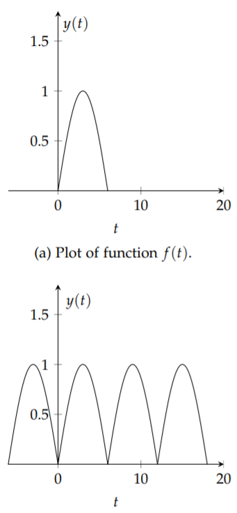
While this appears restrictive, we could also consider functions that are defined over one period. In Figure \(\PageIndex{1}\) we show a function defined on \([0, 2π]\). In the same figure, we show its periodic extension. These are just copies of the original function shifted by the period and glued together. The extension can now be represented by a Fourier series and restricting the Fourier series to \([0, 2π]\) will give a representation of the original function. Therefore, we will first consider Fourier series representations of functions defined on this interval. Note that we could just as easily considered functions defined on \([−π, π]\) or any interval of length \(2π\). We will consider more general intervals later in the chapter.
The Fourier series representation of \(f(x)\) defined on \([0, 2π]\), when it exists, is given by \(\eqref{eq:1}\) with Fourier coefficients
\[\begin{align}a_n&=\frac{1}{\pi}\int_0^{2\pi} f(x)\cos nxdx,\quad n=0,1,2,\ldots ,\nonumber \\ b_n&=\frac{1}{\pi}\int_0^{2\pi}f(x)\sin nxdx,\quad n=1,2,\ldots\label{eq:2}\end{align} \]
These expressions for the Fourier coefficients are obtained by considering special integrations of the Fourier series. We will now derive the \(a_n\) integrals in \(\eqref{eq:2}\).
We begin with the computation of \(a_0\). Integrating the Fourier series term by term in Equation \(\eqref{eq:1}\), we have
\[\label{eq:3}\int_0^{2\pi}f(x)dx=\int_0^{2\pi}\frac{a_0}{2}dx+\int_0^{2\pi}\sum\limits_{n=1}^\infty [a_n\cos nx+b_n\sin nx]dx. \]
Evaluating the integral of an infinite series by integrating term by term depends on the convergence properties of the series.
We will assume that we can integrate the infinite sum term by term. Then we will need to compute
\[\begin{align}\int_0^{2\pi}\frac{a_0}{2}dx&=\frac{a_0}{2}(2\pi )=\pi a_0,\nonumber \\ \int_0^{2\pi}\cos nxdx&=\left[\frac{\sin nx}{n}\right]_0^{2\pi}=0,\nonumber \\ \int_0^{2\pi}\sin nxdx&=\left[\frac{-\cos nx}{n}\right]_0^{2\pi}=0.\label{eq:4}\end{align} \]
From these results we see that only one term in the integrated sum does not vanish leaving
\[\int_0^{2\pi}f(x)dx=\pi a_0.\nonumber \]
This confirms the value for \(a_0\).\(^{2}\)
Next, we will find the expression for \(a_n\). We multiply the Fourier series \(\eqref{eq:1}\) by \(\cos mx\) for some positive integer \(m\). This is like multiplying by \(\cos 2x,\: \cos 5x,\) etc. We are multiplying by all possible \(\cos mx\) functions for different integers \(m\) all at the same time. We will see that this will allow us to solve for the \(a_n\)’s.
We find the integrated sum of the series times \(\cos mx\) is given by
\[ \int_0^{2\pi}f(x)\cos mxdx =\int_0^{2\pi}\frac{a_0}{2}\cos mxdx +\int_0^{2\pi}\sum\limits_{n=1}^\infty [a_n\cos nx+b_n\sin nx]\cos mxdx.\label{eq:5} \]
Integrating term by term, the right side becomes
\[\label{eq:6}\int_0^{2\pi}f(x)\cos mxdx=\frac{a_0}{2}\int_0^{2\pi}\cos mxdx +\sum\limits_{n=1}^\infty\left[a_n\int_0^{2\pi}\cos nx\cos mxdx+b_n\int_0^{2\pi}\sin nx\cos mxdx\right]. \]
We have already established that \(\int_0^{2\pi}\cos mxdx=0\), which implies that the first term vanishes.
Next we need to compute integrals of products of sines and cosines. This requires that we make use of some of the trigonometric identities listed in Chapter 1. For quick reference, we list these here.
\[\begin{align} \sin(x\pm y)&=\sin x\cos y\pm\sin y\cos x\label{eq:7} \\ \cos (x\pm y)&=\cos x\cos y\mp\sin x\sin y \label{eq:8} \\ \sin^2x&=\frac{1}{2}(1-\cos 2x)\label{eq:9} \\ \cos^2x&=\frac{1}{2}(1+\cos 2x)\label{eq:10} \\ \sin x\sin y&=\frac{1}{2}(\cos (x-y)-\cos (x+y))\label{eq:11} \\ \cos x\cos y&=\frac{1}{2}(\cos (x+y)+\cos (x-y))\label{eq:12} \\ \sin x\cos y&=\frac{1}{2}(\sin (x+y)+\sin (x-y))\label{eq:13}\end{align} \]
We first want to evaluate \(\int_0^{2\pi}\cos nx\cos mxdx\). We do this by using the product identity \(\eqref{eq:12}\). We have
\[\begin{align}\int_0^{2\pi}\cos nx\cos mx dx&=\frac{1}{2}\int_0^{2\pi} [\cos (m+n)x+\cos (m-n)x]dx\nonumber \\ &=\frac{1}{2}\left[\frac{\sin (m+n)x}{m+n}+\frac{\sin (m-n)x}{m-n}\right]_0^{2\pi}\nonumber \\ &=0.\label{eq:14}\end{align} \]
There is one caveat when doing such integrals. What if one of the denominators \(m ± n\) vanishes? For this problem \(m + n\neq 0\), since both \(m\) and \(n\) are positive integers. However, it is possible for \(m = n\). This means that the vanishing of the integral can only happen when \(m\neq n\). So, what can we do about the \(m = n\) case? One way is to start from scratch with our integration. (Another way is to compute the limit as \(n\) approaches \(m\) in our result and use L’Hopital’s Rule. Try it!)
For \(n = m\) we have to compute \(\int_0^{2\pi}\cos^2 mx dx\). This can also be handled using a trigonometric identity. Using the half angle formula, \(\eqref{eq:10}\), with \(θ = mx\), we find
\[\begin{align}\int_0^{2\pi}\cos^2mxdx&=\frac{1}{2}\int_0^{2\pi}(1+\cos 2mx)dx\nonumber \\ &=\frac{1}{2}\left[x+\frac{1}{2m}\sin 2mx\right]_0^{2\pi}\nonumber \\ &=\frac{1}{2}(2\pi )=\pi .\label{eq:15}\end{align} \]
To summarize, we have shown that
\[\label{eq:16}\int_0^{2\pi}\cos nx\cos mxdx=\left\{\begin{array}{cc}0,&m\neq n \\ \pi ,&m=n.\end{array}\right. \]
This holds true for \(m, n = 0, 1,\ldots\). [Why did we include \(m, n = 0\)?] When we have such a set of functions, they are said to be an orthogonal set over the integration interval. A set of (real) functions \(\{\phi_n(x)\}\) is said to be orthogonal on \([a, b]\) if \(\int_a^b \phi_n(x)\phi_m(x) dx = 0\) when \(n\neq m\). Furthermore, if we also have that \(\int_a^b \phi_n^2 (x) dx = 1\), these functions are called orthonormal.
The set of functions \(\{cos nx\}_{n=0}^∞\) are orthogonal on \([0, 2π]\). Actually, they are orthogonal on any interval of length \(2π\). We can make them orthonormal by dividing each function by \(\sqrt{\pi}\) as indicated by Equation \(\eqref{eq:15}\). This is sometimes referred to normalization of the set of functions.
The notion of orthogonality is actually a generalization of the orthogonality of vectors in finite dimensional vector spaces. The integral \(\int_a^b f(x)f(x) dx\) is the generalization of the dot product, and is called the scalar product of \(f(x)\) and \(g(x)\), which are thought of as vectors in an infinite dimensional vector space spanned by a set of orthogonal functions. We will return to these ideas in the next chapter.
Returning to the integrals in equation \(\eqref{eq:6}\), we still have to evaluate \(\int_0^{2\pi}\sin nx \cos mx dx\). We can use the trigonometric identity involving products of sines and cosines, \(\eqref{eq:13}\). Setting \(A = nx\) and \(B = mx\), we find that
\[\begin{align}\int_0^{2\pi}\sin nx\cos mxdx&=\frac{1}{2}\int_0^{2\pi}[\sin (n+m)x+\sin (n-m)x]dx\nonumber \\ &=\frac{1}{2}\left[\frac{-\cos (n+m)x}{n+m}+\frac{-\cos (n-m)x}{n-m}\right]_0^{2\pi}\nonumber \\ &=(-1+1)+(-1+1)=0.\label{eq:17}\end{align} \]
So,
\[\label{eq:18}\int_0^{2\pi}\sin nx\cos mxdx=0. \]
For these integrals we also should be careful about setting \(n = m\). In this special case, we have the integrals
\[\int_0^{2\pi}\sin mx\cos mxdx=\frac{1}{2}\int_0^{2\pi}\sin 2mxdx=\frac{1}{2}\left[\frac{-\cos 2mx}{2m}\right]_0^{2\pi}=0.\nonumber \]
Finally, we can finish evaluating the expression in Equation \(\eqref{eq:6}\). We have determined that all but one integral vanishes. In that case, \(n = m\). This leaves us with
\[\int_0^{2\pi}f(x)\cos mxdx=a_m\pi .\nonumber \]
Solving for \(a_m\) gives
\[a_m=\frac{1}{\pi}\int_0^{2\pi}f(x)\cos mxdx.\nonumber \]
Since this is true for all \(m = 1, 2,\ldots\), we have proven this part of the theorem. The only part left is finding the \(b_n\)’s This will be left as an exercise for the reader.
We now consider examples of finding Fourier coefficients for given functions. In all of these cases we define \(f(x)\) on \([0, 2π]\).
\(f(x)=3\cos 2x,\:x\in [0,2\pi ]\).
Solution
We first compute the integrals for the Fourier coefficients.
\[\begin{align}a_0&=\frac{1}{\pi}\int_0^{2\pi}3\cos 2xdx=0.\nonumber \\ a_n&=\frac{1}{\pi}\int_0^{2\pi}3\cos 2x\cos nxdx=0,\quad n\neq 2.\nonumber \\ a_2&=\frac{1}{\pi}\int_0^{2\pi}3\cos^2 2xdx=3,\nonumber \\ b_n&=\frac{1}{\pi}\int_0^{2\pi}3\cos 2x\sin nxdx=0,\quad\forall n.\label{eq:19}\end{align} \]
The integrals for \(a_0, a_n,\: n\neq 2\), and \(b_n\) are the result of orthogonality. For \(a_2\), the integral can be computed as follows:
\[\begin{align}a_2&=\frac{1}{\pi}\int_0^{2\pi}3\cos^2 2xdx\nonumber \\ &=\frac{3}{2\pi}\int_0^{2\pi}[1+\cos 4x]dx\nonumber \\ &=\frac{3}{2\pi}\left[x+\underset{\text{This term vanishes!}}{\underbrace{\frac{1}{4}\sin 4x}}\right]_0^{2\pi}=3.\label{eq:20}\end{align} \]
Therefore, we have that the only nonvanishing coefficient is \(a_2 = 3\). So there is one term and \(f(x) = 3 \cos 2x\).
Well, we should have known the answer to the last example before doing all of those integrals. If we have a function expressed simply in terms of sums of simple sines and cosines, then it should be easy to write down the Fourier coefficients without much work. This is seen by writing out the Fourier series,
\[\begin{align}f(x)&\sim \frac{a_0}{2}+\sum\limits_{n=1}^\infty [a_n\cos nx+b_n\sin nx].\nonumber \\ &=\frac{a_0}{2}+a_1\cos x+b_1\sin x+a_2\cos 2x+b_2\sin 2x+\cdots\label{eq:21}\end{align} \]
For the last problem, \(f(x) = 3 \cos 2x\). Comparing this to the expanded Fourier series, one can immediately read off the Fourier coefficients without doing any integration. In the next example we emphasize this point.
\(f(x)=\sin^2x,\: x\in [0,2\pi ]\).
Solution
We could determine the Fourier coefficients by integrating as in the last example. However, it is easier to use trigonometric identities. We know that
\[\sin^2x=\frac{1}{2}(1-\cos 2x)=\frac{1}{2}-\frac{1}{2}\cos 2x.\nonumber \]
There are no sine terms, so \(b_n = 0,\) \(n = 1, 2,\ldots\). There is a constant term, implying \(a_0/2 = 1/2\). So, \(a_0 = 1\). There is a \(\cos 2x\) term, corresponding to \(n = 2\), so \(a_2 = −\frac{1}{2}\). That leaves \(a_n = 0\) for \(n\neq 0, 2\). So, \(a_0 = 1,\: a_2 = −\frac{1}{2}\), and all other Fourier coefficients vanish.
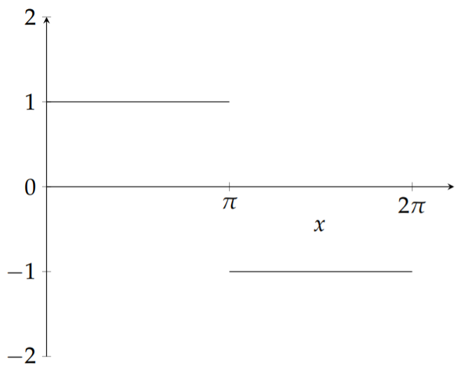
\(f(x)=\left\{\begin{array}{cc}1,&0<x<\pi , \\ -1, &\pi <x<2\pi ,\end{array}\right.\)
Solution
This example will take a little more work. We cannot bypass evaluating any integrals this time. As seen in Figure \(\PageIndex{2}\), this function is discontinuous. So, we will break up any integration into two integrals, one over \([0, π]\) and the other over \([π, 2π]\).
\[\begin{align}a_0&=\frac{1}{\pi}\int_0^{2\pi}f(x)dx\nonumber \\ &=\frac{1}{\pi}\int_0^{\pi}dx+\frac{1}{\pi}\int_\pi^{2\pi}(-1)dx\nonumber \\ &=\frac{1}{\pi}(\pi )+\frac{1}{\pi}(-2\pi +\pi )=0.\label{eq:22}\end{align} \]
\[\begin{align}a_n&=\frac{1}{\pi}\int_0^{2\pi}f(x)\cos nxdx\nonumber \\ &=\frac{1}{\pi}\left[\int_0^\pi \cos nxdx-\int_\pi^{2\pi}\cos nxdx\right] \nonumber \\ &=\frac{1}{\pi}\left[\left(\frac{1}{n}\sin nx\right)_0^{\pi}-\left(\frac{1}{n}\sin nx\right)_\pi^{2\pi}\right]\nonumber \\ &=0.\label{eq:23}\end{align} \]
\[\begin{align}b_n&=\frac{1}{\pi}\int_0^{2\pi}f(x)\sin nxdx\nonumber \\ &=\frac{1}{\pi}\left[\int_0^\pi \sin nxdx-\int_\pi^{2\pi}\sin nxdx\right]\nonumber \\ &=\frac{1}{\pi}\left[\left(-\frac{1}{n}\cos nx\right)_0^\pi +\left(\frac{1}{n}\cos nx\right)_\pi^{2\pi}\right]\nonumber \\ &=\frac{1}{\pi}\left[-\frac{1}{n}\cos n\pi +\frac{1}{n}+\frac{1}{n}-\frac{1}{n}\cos n\pi\right]\nonumber \\ &=\frac{2}{n\pi}(1-\cos n\pi ).\label{eq:24}\end{align} \]
Often we see expressions involving \(\cos nπ = (−1)^n\) and \(1 ± \cos nπ = 1 ± (−1)^n\). This is an example showing how to re-index series containing \(\cos nπ\).
We have found the Fourier coefficients for this function. Before inserting them into the Fourier series \(\eqref{eq:1}\), we note that \(\cos nπ = (−1)^n\). Therefore,
\[\label{eq:25}1-\cos n\pi=\left\{\begin{array}{cl}0,&n\text{ even} \\ 2,&n\text{ odd.}\end{array}\right. \]
So, half of the \(b_n\)’s are zero. While we could write the Fourier series representation as
\[f(x)\sim\frac{4}{\pi}\sum\limits_{\underset{n\text{ odd}}{n=1}}^\infty \frac{1}{n}\sin nx,\nonumber \]
we could let \(n = 2k − 1\) in order to capture the odd numbers only. The answer can be written as
\[f(x)=\frac{4}{\pi}\sum\limits_{k=1}^\infty\frac{\sin (2k-1)x}{2k-1}.\nonumber \]
Having determined the Fourier representation of a given function, we would like to know if the infinite series can be summed; i.e., does the series converge? Does it converge to \(f(x)\)? We will discuss this question later in the chapter after we generalize the Fourier series to intervals other than for \(x ∈ [0, 2π]\).