3.6: Finite Length Strings

We now return to the physical example of wave propagation in a string. We found that the general solution can be represented as a sum over product solutions. We will restrict our discussion to the special case that the initial velocity is zero and the original profile is given by $u(x, 0)=f(x)$. The solution is then

$$u(x, t)=\sum_{n=1}^{\infty} A_{n} \sin \frac{n \pi x}{L} \cos \frac{n \pi c t}{L}\label{eq:1}$$

satisfying

$$f(x)=\sum_{n=1}^{\infty} A_{n} \sin \frac{n \pi x}{L} .\label{eq:2}$$

We have seen that the Fourier sine series coefficients are given by

$$A_{n}=\frac{2}{L} \int_{0}^{L} f(x) \sin \frac{n \pi x}{L} d x .\label{eq:3}$$

We can rewrite this solution in a more compact form. First, we define the wave numbers,

$$k_{n}=\frac{n \pi}{L}, \quad n=1,2, \ldots,\nonumber$$

and the angular frequencies,

$$\omega_{n}=c k_{n}=\frac{n \pi c}{L} .\nonumber$$

Then, the product solutions take the form

$$\sin k_{n} x \cos \omega_{n} t\nonumber$$

Using trigonometric identities, these products can be written as

$$\sin k_{n} x \cos \omega_{n} t=\frac{1}{2}\left[\sin \left(k_{n} x+\omega_{n} t\right)+\sin \left(k_{n} x-\omega_{n} t\right)\right] .\nonumber$$

Inserting this expression in the solution, we have

$$u(x, t)=\frac{1}{2} \sum_{n=1}^{\infty} A_{n}\left[\sin \left(k_{n} x+\omega_{n} t\right)+\sin \left(k_{n} x-\omega_{n} t\right)\right] .\label{eq:4}$$

Since $\omega_{n}=c k_{n}$, we can put this into a more suggestive form:

$$u(x, t)=\frac{1}{2}\left[\sum_{n=1}^{\infty} A_{n} \sin k_{n}(x+c t)+\sum_{n=1}^{\infty} A_{n} \sin k_{n}(x-c t)\right] .\label{eq:5}$$

We see that each sum is simply the sine series for $f(x)$ but evaluated at either $x+c t$ or $x-c t$. Thus, the solution takes the form

$$u(x, t)=\frac{1}{2}[f(x+c t)+f(x-c t)] .\label{eq:6}$$

If $t=0$, then we have $u(x, 0)=\frac{1}{2}[f(x)+f(x)]=f(x)$. So, the solution satisfies the initial condition. At $t=1$, the sum has a term $f(x-c)$.

Recall from your mathematics classes that this is simply a shifted version of $f(x)$. Namely, it is shifted to the right. For general times, the function is shifted by $c t$ to the right. For larger values of $t$, this shift is further to the right. The function (wave) shifts to the right with velocity $c$. Similarly, $f(x+c t)$ is a wave traveling to the left with velocity $-c$.

Thus, the waves on the string consist of waves traveling to the right and to the left. However, the story does not stop here. We have a problem when needing to shift $f(x)$ across the boundaries. The original problem only defines $f(x)$ on $[0, L]$. If we are not careful, we would think that the function leaves the interval leaving nothing left inside. However, we have to recall that our sine series representation for $f(x)$ has a period of $2 L$. So, before we apply this shifting, we need to account for its periodicity. In fact, being a sine series, we really have the odd periodic extension of $f(x)$ being shifted. The details of such analysis would take us too far from our current goal. However, we can illustrate this with a few figures.

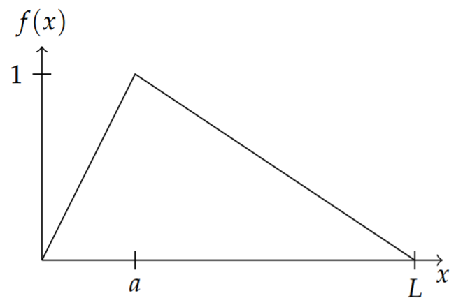
We begin by plucking a string of length $L$. This can be represented by the function

$$f(x)=\left\{\begin{array}{cc} \frac{x}{a} & 0 \leq x \leq a \\ \frac{L-x}{L-a} & a \leq x \leq L \end{array}\right.\label{eq:7}$$

where the string is pulled up one unit at $x=a$. This is shown in Figure $\PageIndex{1}$.

Figure $\PageIndex{1}$: The initial profile for a string of length one plucked at $x=a$.

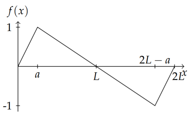
Next, we create an odd function by extending the function to a period of $2 L$. This is shown in Figure $\PageIndex{2}$.

Figure $\PageIndex{2}$: Odd extension about the right end of a plucked string.

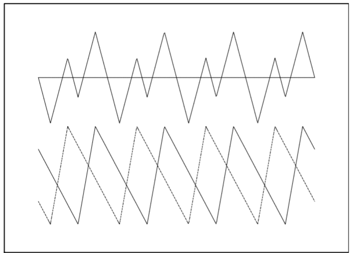
Finally, we construct the periodic extension of this to the entire line. In Figure $\PageIndex{3}$ we show in the lower part of the figure copies of the periodic extension, one moving to the right and the other moving to the left. (Actually, the copies are $\frac{1}{2} f(x \pm c t)$.) The top plot is the sum of these solutions. The physical string lies in the interval $[0,1]$. Of course, this is better seen when the solution is animated.

Figure $\PageIndex{3}$: Summing the odd periodic extensions. The lower plot shows copies of the periodic extension, one moving to the right and the other moving to the left. The upper plot is the sum.

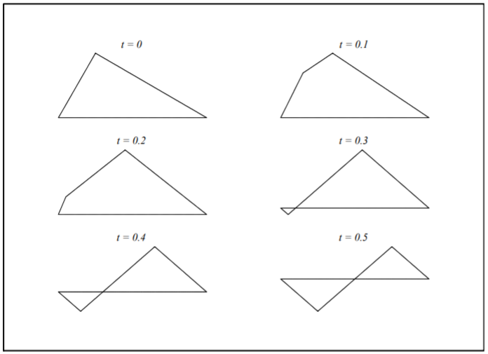
The time evolution for this plucked string is shown for several times in Figure $\PageIndex{4}$. This results in a wave that appears to reflect from the ends as time increases.

Figure $\PageIndex{4}$: This Figure shows the plucked string at six successive times.

The relation between the angular frequency and the wave number, $\omega=$ $c k$, is called a dispersion relation. In this case $\omega$ depends on $k$ linearly. If one knows the dispersion relation, then one can find the wave speed as $c=\frac{\omega}{k}$. In this case, all of the harmonics travel at the same speed. In cases where they do not, we have nonlinear dispersion, which we will discuss later.