17.2: Projective model

The following picture illustrates the map \(P\mapsto \hat{P}\) described in the previous section — if you take the picture on the left and apply the map \(P\mapsto \hat P\), you get the picture on the right. The pictures are conformal and projective model of the hyperbolic plane respectively. The map \(P\mapsto \hat P\) is a “translation” from one to another.

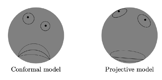
In the projective model things look different; some become simpler, other things become more complicated.

Lines

The h-lines in the projective model are chords of the absolute; more precisely, chords without its endpoints.

This observation can be used to transfer statements about lines and points from the Euclidean plane to the h-plane. As an example let us state a hyperbolic version of Pappus’ theorem for h-plane.

Theorem \(\PageIndex{1}\) Hyperbolic Pappus' theorem

Assume that two triples of h-points \(A\), \(B\), \(C\), and \(A'\), \(B'\), \(C'\) in the h-plane are h-collinear. Suppose that the h-points \(X\), \(Y\), and \(Z\) are defined by

\(\begin{aligned} X&=(BC')_h\cap(B'C)_h, & Y&=(CA')_h\cap(C'A)_h, & Z&=(AB')_h \cap(A'B)_h.\end{aligned}\)

Then the points \(X\), \(Y\), \(Z\) are h-collinear.

In the projective model, this statement follows immediately from the original Pappus’ theorem 15.6.2. The same can be done for Desargues’ theorem 15.6.1. The same argument shows that the construction of a tangent line with a ruler only described in Exercise 15.8.2 works in the h-plane as well.

On the other hand, note that it is not at all easy to prove this statement using the conformal model.

Circles and equidistants

The h-circles and equidistants in the projective model are certain type of ellipses and their open arcs.

It follows since the stereographic projection sends circles on the plane to circles on the unit sphere and the foot point projection of the circle back to the plane is an ellipse. (One may define ellipse as a foot point projection of a circle.)

Distance

Consider a pair of h-points \(P\) and \(Q\). Let \(A\) and \(B\) be the ideal point of the h-line in projective model; that is, \(A\) and \(B\) are the intersections of the Euclidean line \((PQ)\) with the absolute.

Then by Lemma 17.1.1,

assuming the points \(A, P, Q, B\) appear on the line in the same order.

Angles

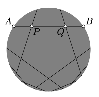
The angle measures in the projective model are very different from the Euclidean angles and it is hard to figure out by looking on the picture.(The idea described in the solution of Exercise 16.3.1 and in the sketch of proof of Theorem 19.4.1 can be used to construct many projective transformations of this type.) For example all the intersecting h-lines on the picture are perpendicular.

There are two useful exceptions:

• If \(O\) is the center of the absolute, then \[\measuredangle_hAOB=\measuredangle AOB.\]
• If \(O\) is the center of the absolute and \(\measuredangle OAB=\pm\tfrac\pi2\), then

\(\measuredangle_h OAB=\measuredangle OAB=\pm \dfrac{\pi}{2}.\)

To find the angle measure in the projective model, you may apply a motion of the h-plane that moves the vertex of the angle to the center of the absolute; once it is done the hyperbolic and Euclidean angles have the same measure.

Motions

The motions of the h-plane in the conformal and projective models are relevant to inversive transformations and projective transformation in the same way. Namely:

• Inversive transformations that preserve the h-plane describe motions of the h-plane in the conformal model.
• Projective transformations that preserve h-plane describe motions of the h-plane in the projective model.¹

The following exercise is a hyperbolic analog of Exercise 16.5.1. This is the first example of a statement that admits an easier proof using the projective model.

Exercise \(\PageIndex{1}\)

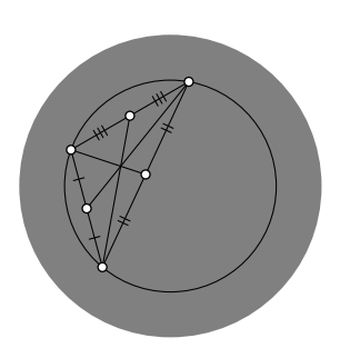
Let \(P\) and \(Q\) be the points in h-plane that lie on the same distance from the center of the absolute. Observe that in the projective model, h-midpoint of \([PQ]_h\) coincides with the Euclidean midpoint of \([PQ]_h\).

Conclude that if an h-triangle is inscribed in an h-circle, then its medians meet at one point.

Recall that an h-triangle might be also inscribed in a horocycle or an equidistant. Think how to prove the statement in this case.

Hint

The observation follows since the reflection across the perpendicular bisector of \([PQ]\) is a motion of the Euclidean plane, and a motion of the h-plane as well. Without loss of generality, we may assume that the center of the circumcircle coincides with the center of the absolute. In this case the h-medians of the triangle coincide with the Euclidean medians. It remains to apply Theorem 8.3.1.

Exercise \(\PageIndex{2}\)

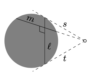
Let \(\ell\) and \(m\) are h-lines in the projective model. Let \(s\) and \(t\) denote the Euclidean lines tangent to the absolute at the ideal points of \(\ell\). Show that if the lines \(s\), \(t\) and the extension of \(m\) intersect at one point, then \(\ell\) and \(m\) are perpendicular h-lines.

Hint

Let \(\hat{\ell}\) and \(\hat{m}\) denote the h-lines in the conformal model that correspond to \(\ell\) and \(m\). We need to show that \(\hat{\ell} \perp \hat{m}\) as arcs in the Euclidean plane.

The point \(Z\), where \(s\) meets \(t\), is the center of the circle \(\Gamma\) containing \(\hat{\ell}\).

If \(\hat{m}\) is passing thru \(Z\), then the inversion in \(\Gamma\) exchange the ideal points of \(\hat{\ell}\). In particular, \(\hat{\ell}\) maps to itself. Hence the result.

Exercise \(\PageIndex{3}\)

Use the projective model to derive the formula for angle of parallelism (Proposition 13.1.1).

Hint

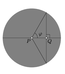
Let \(Q\) be the foot point of \(P\) on the line and \(\varphi\) be the angle of parallelism. We can assume that \(P\) is the center of the absolute. Therefore \(PQ = \cos \varphi\) and

\(PQ_h = \dfrac{1}{2} \cdot \ln \dfrac{1 + \cos \varphi}{1 - \cos \varphi}.\)

Exercise \(\PageIndex{4}\)

Use projective model to find the in radius of the ideal triangle.

Hint

Apply Exercise \(\PageIndex{3}\) for \(\varphi = \dfrac{\pi}{3}\).

The projective model of h-plane can be used to give another proof of the hyperbolic Pythagorean theorem (Theorem 13.6.1).

First let us recall its statement:

\[\cosh c=\cosh a\cdot\cosh b,\]

where \(a=BC_h\), \(b=CA_h\), and \(c=AB_h\) and \(\triangle_hACB\) is an h-triangle with right angle at \(C\).

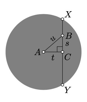
Note that we can assume that \(A\) is the center of the absolute. Set \(s=BC\), \(t =CA\), \(u= AB\). According to the Euclidean Pythagorean theorem (Theorem 6.2.1), we have

\[u^2=s^2+t^2.\]

It remains to express \(a\), \(b\), and \(c\) using \(s\), \(u\), and \(t\) and show that 17.2.3 implies 17.2.2.

Advanced Exercise \(\PageIndex{5}\)

Finish the proof of hyperbolic Pythagorean theorem (Theorem 13.6.1) indicated above.

Hint

Note that \(b = \dfrac{1}{2} \cdot \ln \dfrac{1 + t}{1 - t}\), therefore,

\[\cosh b = \dfrac{1}{2} \cdot (\sqrt{\dfrac{1 + t}{1 - t}} + \sqrt{\dfrac{1 - t}{1 +t}}) = \dfrac{1}{\sqrt{1 - t^2}}.\]

The same way we get that

\[\cosh c = \dfrac{1}{\sqrt{1 - u^2}}.\]

Let \(X\) and \(Y\) are the ideal points of \((BC)_h\). Applying the Pythagorean theorem (Theorem 6.2.1) again, we get that \(CX = CY = \sqrt{1 - t^2}\). Therefore,

\(a = \dfrac{1}{2} \cdot \ln \dfrac{\sqrt{1 - t^2} + s}{\sqrt{1 - t^2} - s},\)

and

\[\cosh a = \dfrac{1}{2} \cdot (\dfrac{\sqrt{1 - t^2} + s}{\sqrt{1 - t^2} - s} + \dfrac{\sqrt{1 - t^2} - s}{\sqrt{1 - t^2} + s}) = \dfrac{\sqrt{1 - t^2}}{\sqrt{1 - t^2 - s^2}} = \dfrac{\sqrt{1 - t^2}}{\sqrt{1 - u^2}}.\]

Finally, note that 17.2.5, 17.2.6, and 17.2.7 imply the theorem.