12.1: Polynomial Inequalities
- Page ID
- 49024
\( \newcommand{\vecs}[1]{\overset { \scriptstyle \rightharpoonup} {\mathbf{#1}} } \)
\( \newcommand{\vecd}[1]{\overset{-\!-\!\rightharpoonup}{\vphantom{a}\smash {#1}}} \)
\( \newcommand{\dsum}{\displaystyle\sum\limits} \)
\( \newcommand{\dint}{\displaystyle\int\limits} \)
\( \newcommand{\dlim}{\displaystyle\lim\limits} \)
\( \newcommand{\id}{\mathrm{id}}\) \( \newcommand{\Span}{\mathrm{span}}\)
( \newcommand{\kernel}{\mathrm{null}\,}\) \( \newcommand{\range}{\mathrm{range}\,}\)
\( \newcommand{\RealPart}{\mathrm{Re}}\) \( \newcommand{\ImaginaryPart}{\mathrm{Im}}\)
\( \newcommand{\Argument}{\mathrm{Arg}}\) \( \newcommand{\norm}[1]{\| #1 \|}\)
\( \newcommand{\inner}[2]{\langle #1, #2 \rangle}\)
\( \newcommand{\Span}{\mathrm{span}}\)
\( \newcommand{\id}{\mathrm{id}}\)
\( \newcommand{\Span}{\mathrm{span}}\)
\( \newcommand{\kernel}{\mathrm{null}\,}\)
\( \newcommand{\range}{\mathrm{range}\,}\)
\( \newcommand{\RealPart}{\mathrm{Re}}\)
\( \newcommand{\ImaginaryPart}{\mathrm{Im}}\)
\( \newcommand{\Argument}{\mathrm{Arg}}\)
\( \newcommand{\norm}[1]{\| #1 \|}\)
\( \newcommand{\inner}[2]{\langle #1, #2 \rangle}\)
\( \newcommand{\Span}{\mathrm{span}}\) \( \newcommand{\AA}{\unicode[.8,0]{x212B}}\)
\( \newcommand{\vectorA}[1]{\vec{#1}} % arrow\)
\( \newcommand{\vectorAt}[1]{\vec{\text{#1}}} % arrow\)
\( \newcommand{\vectorB}[1]{\overset { \scriptstyle \rightharpoonup} {\mathbf{#1}} } \)
\( \newcommand{\vectorC}[1]{\textbf{#1}} \)
\( \newcommand{\vectorD}[1]{\overrightarrow{#1}} \)
\( \newcommand{\vectorDt}[1]{\overrightarrow{\text{#1}}} \)
\( \newcommand{\vectE}[1]{\overset{-\!-\!\rightharpoonup}{\vphantom{a}\smash{\mathbf {#1}}}} \)
\( \newcommand{\vecs}[1]{\overset { \scriptstyle \rightharpoonup} {\mathbf{#1}} } \)
\(\newcommand{\longvect}{\overrightarrow}\)
\( \newcommand{\vecd}[1]{\overset{-\!-\!\rightharpoonup}{\vphantom{a}\smash {#1}}} \)
\(\newcommand{\avec}{\mathbf a}\) \(\newcommand{\bvec}{\mathbf b}\) \(\newcommand{\cvec}{\mathbf c}\) \(\newcommand{\dvec}{\mathbf d}\) \(\newcommand{\dtil}{\widetilde{\mathbf d}}\) \(\newcommand{\evec}{\mathbf e}\) \(\newcommand{\fvec}{\mathbf f}\) \(\newcommand{\nvec}{\mathbf n}\) \(\newcommand{\pvec}{\mathbf p}\) \(\newcommand{\qvec}{\mathbf q}\) \(\newcommand{\svec}{\mathbf s}\) \(\newcommand{\tvec}{\mathbf t}\) \(\newcommand{\uvec}{\mathbf u}\) \(\newcommand{\vvec}{\mathbf v}\) \(\newcommand{\wvec}{\mathbf w}\) \(\newcommand{\xvec}{\mathbf x}\) \(\newcommand{\yvec}{\mathbf y}\) \(\newcommand{\zvec}{\mathbf z}\) \(\newcommand{\rvec}{\mathbf r}\) \(\newcommand{\mvec}{\mathbf m}\) \(\newcommand{\zerovec}{\mathbf 0}\) \(\newcommand{\onevec}{\mathbf 1}\) \(\newcommand{\real}{\mathbb R}\) \(\newcommand{\twovec}[2]{\left[\begin{array}{r}#1 \\ #2 \end{array}\right]}\) \(\newcommand{\ctwovec}[2]{\left[\begin{array}{c}#1 \\ #2 \end{array}\right]}\) \(\newcommand{\threevec}[3]{\left[\begin{array}{r}#1 \\ #2 \\ #3 \end{array}\right]}\) \(\newcommand{\cthreevec}[3]{\left[\begin{array}{c}#1 \\ #2 \\ #3 \end{array}\right]}\) \(\newcommand{\fourvec}[4]{\left[\begin{array}{r}#1 \\ #2 \\ #3 \\ #4 \end{array}\right]}\) \(\newcommand{\cfourvec}[4]{\left[\begin{array}{c}#1 \\ #2 \\ #3 \\ #4 \end{array}\right]}\) \(\newcommand{\fivevec}[5]{\left[\begin{array}{r}#1 \\ #2 \\ #3 \\ #4 \\ #5 \\ \end{array}\right]}\) \(\newcommand{\cfivevec}[5]{\left[\begin{array}{c}#1 \\ #2 \\ #3 \\ #4 \\ #5 \\ \end{array}\right]}\) \(\newcommand{\mattwo}[4]{\left[\begin{array}{rr}#1 \amp #2 \\ #3 \amp #4 \\ \end{array}\right]}\) \(\newcommand{\laspan}[1]{\text{Span}\{#1\}}\) \(\newcommand{\bcal}{\cal B}\) \(\newcommand{\ccal}{\cal C}\) \(\newcommand{\scal}{\cal S}\) \(\newcommand{\wcal}{\cal W}\) \(\newcommand{\ecal}{\cal E}\) \(\newcommand{\coords}[2]{\left\{#1\right\}_{#2}}\) \(\newcommand{\gray}[1]{\color{gray}{#1}}\) \(\newcommand{\lgray}[1]{\color{lightgray}{#1}}\) \(\newcommand{\rank}{\operatorname{rank}}\) \(\newcommand{\row}{\text{Row}}\) \(\newcommand{\col}{\text{Col}}\) \(\renewcommand{\row}{\text{Row}}\) \(\newcommand{\nul}{\text{Nul}}\) \(\newcommand{\var}{\text{Var}}\) \(\newcommand{\corr}{\text{corr}}\) \(\newcommand{\len}[1]{\left|#1\right|}\) \(\newcommand{\bbar}{\overline{\bvec}}\) \(\newcommand{\bhat}{\widehat{\bvec}}\) \(\newcommand{\bperp}{\bvec^\perp}\) \(\newcommand{\xhat}{\widehat{\xvec}}\) \(\newcommand{\vhat}{\widehat{\vvec}}\) \(\newcommand{\uhat}{\widehat{\uvec}}\) \(\newcommand{\what}{\widehat{\wvec}}\) \(\newcommand{\Sighat}{\widehat{\Sigma}}\) \(\newcommand{\lt}{<}\) \(\newcommand{\gt}{>}\) \(\newcommand{\amp}{&}\) \(\definecolor{fillinmathshade}{gray}{0.9}\)We now consider inequalities. Solving inequalities is quite similar to solving equalities. There is one extra consideration, that multiplying or dividing by a negative number on both sides of an inequality changes the direction of the inequality sign.
\[\begin{array}{cccc}
& -2 x \leq-6 & \Longrightarrow & x {\color{Red} \geq } 3 \\
\text { but } & 2 x \leq 6 & \Longrightarrow & x \leq 3
\end{array} \nonumber \]
Solve for \(x\).
- \(-3x+7> 19\)
- \(2x+5\geq 4x-11\)
- \(3 <-6x-4\leq 13\)
- \(-2x-1\leq 3x+4< 4x-20\)
Solution
- \(-3 x+7>19 \quad \stackrel{(-7)}{\Longrightarrow} \quad-3 x>12 \stackrel{(\div(-3))}{\Longrightarrow} \quad x<-4\)
- \(2 x+5 \geq 4 x-11 \stackrel{(-4 x-5)}{\Longrightarrow} \quad-2 x \geq-16 \stackrel{(\div(-2))}{\Longrightarrow} \quad x \leq 8\)
- \[3<-6 x-4 \leq 13 \quad \stackrel{(+4)}{\Longrightarrow} \quad 7<-6 x \leq 17 \quad \stackrel{(\div(-6))}{\Longrightarrow} \quad \dfrac{7}{-6}>x \geq \dfrac{17}{-6} \quad \Longrightarrow \quad-\dfrac{17}{6} \leq x<-\dfrac{7}{6} \nonumber \] The last implication was obtained by switching the right and left terms of the inequality. The solution set is the interval \([-\dfrac{17}{6},-\dfrac{7}{6})\).
- For part (d), it is best to consider both inequalities separately.
\[\begin{aligned} -2x-1\leq 3x+4 \quad \stackrel{(-3x+1)} \implies \quad -5x\leq 5 \stackrel{(\div(-5))} \implies \quad x\geq -1 \\ 3x+4< 4x-20 \quad\stackrel{(-4x-4)} \implies \quad -x<-24 \stackrel{(\cdot(-1))} \implies \quad x> 24\end{aligned} \nonumber \]
The solution has to satisfy both inequalities \(x\geq -1\) and \(x>24\). Both inequalities are true for \(x>24\) (since then also \(x\geq -1\)), so that this is in fact the solution: \(x>24\).
When dealing with polynomial inequalities, we use the same three-step strategy that we used in section 1.4. More precisely, the first step is to solve the corresponding equality, and the second step is to determine the solution by investigating the subintervals induced from step 1. For both of these steps we may now also use the graph of the function and its display on the graphing calculator. The third step is to check the endpoints of each interval.
Solve for \(x\).
- \(x^2-3x-4\geq 0\)
- \(x^3-9x^2+23x-15\leq 0\)
- \(x^4-x^2 > 5(x^3-x)\)
- \(x^3+15x>7x^2+9\)
- \(x^5-6x^4-26x^3+144x^2-47x-210\leq 0\)
Solution
- We can find the roots of the polynomial on the left by factoring.
\[x^2-3x-4=0 \implies \quad (x-4)(x+1)=0 \implies \quad x=4 \text{ or }x=-1 \nonumber \]
To see where \(f(x)=x^2-3x-4\) is \(\geq 0\), we graph it with the calculator.
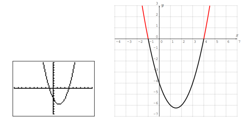
We see that \(f(x)\geq 0\) when \(x\leq -1\) and when \(x\geq 4\) (the parts of the graph above the \(x\)-axis). The solution set is therefore
\[\{x|x\leq -1,\text{ or }x\geq 4\}=(-\infty,-1]\cup [4,\infty) \nonumber \]
- Here is the graph of the function \(f(x)=x^3-9x^2+23x-15\) with the TI-84 in the standard window.
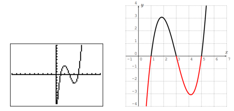
This graph shows that there are two intervals where \(f(x)\leq 0\) (the parts of the graph below the \(x\)-axis). To determine the exact intervals, we calculate where \(f(x)=x^3-9x^2+23x-15=0\). The graph suggests that the roots of \(f(x)\) are at \(x=1\), \(x=3\), and \(x=5\). This can be confirmed by a calculation:
\[\begin{aligned} f(1)&= 1^3-9\cdot 1^2+23\cdot 1-15=1-9+23-15=0\\ f(3)&= 3^3-9\cdot 3^2+23\cdot 3-15=27-81+69-15=0\\ f(5)&= 5^3-9\cdot 5^2+23\cdot 5-15=125-225+115-15=0\end{aligned} \nonumber \]
Since \(f\) is a polynomial of degree \(3\), the roots \(x=1, 3, 5\) are all of the roots of \(f\). (Alternatively, we could have divided \(f(x)\), for example, by \(x-1\) and used this to completely factor \(f\) and with this obtain all the roots of \(f\).) With this, we can determine the solution set to be the set:
\[\begin{aligned} \text{solution set}&=\{x\in \mathbb{R} | x\leq 1, \text{ or } 3\leq x\leq 5\} \\ &=(-\infty,1]\cup [3,5] \end{aligned} \nonumber \]
Note that we include the roots \(1\), \(3\), and \(5\) in the solution set since the original inequality was “\(\leq\)” (and not “\(<\)”), which includes the solutions of the corresponding equality.
- In order to use the graphing calculator, we rewrite the inequality to obtain zero on one side of the inequality.
\[\begin{aligned}
x^{4}-x^{2}>5\left(x^{3}-x\right) (\text { distribute } 5) & \Longrightarrow \quad x^{4}-x^{2}>5 x^{3}-5 x \\
\left(\text { subtract } 5 x^{3}, \text{ add } 5 x\right) & \Longrightarrow \quad x^{4}-5 x^{3}-x^{2}+5 x>0
\end{aligned} \nonumber \]
We graph \(f(x)=x^4-5x^3-x^2+5x\) with the TI-84.
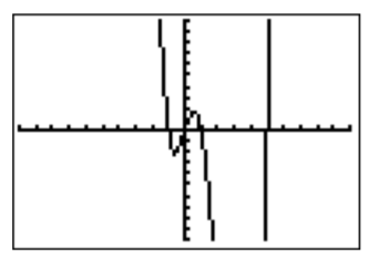
The graph suggests the roots \(x=-1\), \(0\), \(1\), and \(5\). This can be confirmed by a straightforward calculation.
\[\begin{aligned} f(-1)&= (-1)^4-5\cdot (-1)^3-(-1)^2+5\cdot (-1)=1+5-1-5=0\\ f(0)&= 0^4-5\cdot 0^3-0^2-5\cdot 0=0\\ f(1)&= 1^4-5\cdot 1^3-1^2+5\cdot 1=1-5-1+5=0\\ f(5)&= 5^4-5\cdot 5^3-5^2+5\cdot 5=125-125-25+25=0\end{aligned} \nonumber \]
The roots \(x=-1\), \(0\), \(1\), and \(5\) are the only roots since \(f\) is of degree \(4\). The intervals of the solution for \(f(x)>0\) may be read off from the graph:
\[\text{solution set}=(-\infty,-1)\cup (0,1)\cup (5, \infty) \nonumber \]
(Notice that the roots \(-1\), \(0\), \(1\), and \(5\) are not included in the solution set since our inequality reads \(f(x)>0\) and not \(f(x)\geq 0\).)
- Again, we bring all terms to one side:
\[x^3+15x>7x^2+9 \implies x^3-7x^2+15x-9>0 \nonumber \]
(Here it does not matter whether we bring the terms to the right or the left side of the inequality sign! The resulting inequality is different, but the solution to the problem is the same.) With this, we now use the TI-84 to find the graph of the function \(f(x)=x^3-7x^2+15x-9\).
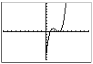
The graph suggests at least one root (the left most intersection point), but possibly one or two more roots. To gain a better understanding of whether the graph intersects the \(x\)-axis on the right, we rescale the window size of the previous graph.
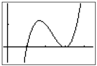
This viewing window suggests that there are two roots \(x=1\) and \(x=3\). We confirm that these are the only roots with an algebraic computation. First, we check that \(x=1\) and \(x=3\) are indeed roots:
\[\begin{aligned} f(1)&= 1^3-7\cdot 1^2+15\cdot 1-9=1-7+15-9=0\\ f(3)&= 3^3-7\cdot 3^2+15\cdot 3-9=27-63+45-9=0\end{aligned}\]
To confirm that these are the only roots (and we have not just missed one of the roots which might possibly become visible after sufficiently zooming into the graph), we factor \(f(x)\) completely. We divide \(f(x)\) by \(x-1\):
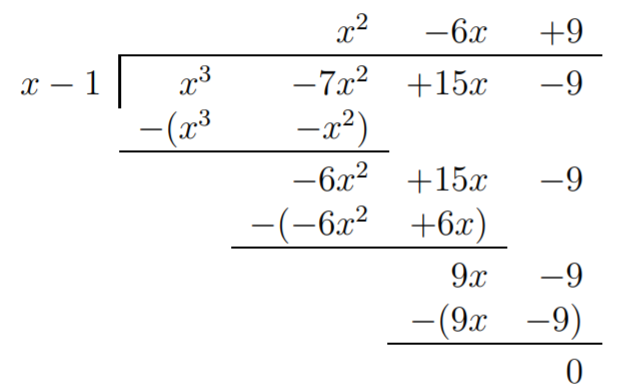
and use this to factor \(f\):
\[\begin{aligned} f(x)&= x^3-7x^2+15x-9 = (x-1)(x^2-6x+9) \\ &= (x-1)(x-3)(x-3)\end{aligned} \nonumber \]
This shows, that \(3\) is a root of multiplicity \(2\), and so \(f\) has no other roots than \(x=1\) and \(x=3\). The solution set consists of those numbers \(x\) for which \(f(x)>0\). From the graph we see that this is the case when \(1<x<3\) and when \(x>3\) (the roots \(x=1\) and \(x=3\) are not included as solutions). We can write the solution set in several different ways:
\[\text{solution set}= \{x | 1<x<3 \text{ or } x>3 \} = \{x|1<x\}-\{3\} \nonumber \]
or in interval notation:
\[\text{solution set}= (1,3)\cup (3,\infty) = (1,\infty)-\{3\} \nonumber \]
- If we set \(f(x)=x^5-6x^4-26x^3+144x^2-47x-210\) then we need to find those numbers \(x\) with \(f(x)\leq 0\). We first graph \(f\) in the standard window.
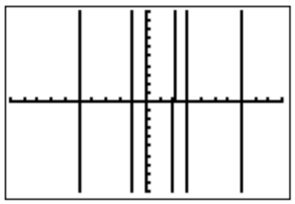
To get a better view of the graph, we rescale to an appropriate window:

There appear to be three intervals, where \(f(x)\leq 0\). To determine the exact numbers, we guess some of the roots from the graph. These would be \(x=-5, -1, 2, 3, 7\). To confirm these roots, we calculate the following function values.
\[\begin{aligned} f(-5)&= (-5)^5-6\cdot (-5)^4-26 \cdot (-5)^3+144\cdot (-5)^2-47\cdot (-5)-210\\ &= -3125-3750+3250+3600+235-210=0 \\ f(-1)&= (-1)^5-6\cdot (-1)^4-26 \cdot (-1)^3+144\cdot (-1)^2-47\cdot (-1)-210\\ &= -1-6+26+576+47-210=0\\ f(2)&= 2^5-6\cdot 2^4-26 \cdot 2^3+144\cdot 2^2-47\cdot 2-210\\ &= 32-96-208+576-94-210=0\\ f(3)&= 3^5-6\cdot 3^4-26 \cdot 3^3+144\cdot 3^2-47\cdot 3-210\\ &= 243-486-702+1296-141-210=0\\ f(7)&= 7^5-6\cdot 7^4-26 \cdot 7^3+144\cdot 7^2-47\cdot 7-210\\ &= 16807-14406-8918+7056-329-210=0\end{aligned} \nonumber \]
Since \(f(x)\) is of degree \(5\), we know that these are all of the roots of \(f(x)\). The solution set for \(f(x)\leq 0\) can be read from the graphs above:
\[\text{solution set}=(-\infty,-5]\cup [-1,2]\cup [3,7] \nonumber \]
(Note again, that the roots are all included in the solution set.)
Polynomial inequalities come up, for example, when finding the domain of functions involving a square root, as we will show in the next example.
Find the domain of the given functions.
- \( f(x)=\sqrt{x^2-4}\)
- \(g(x)=\sqrt{x^3-5x^2+6x}\)
Solution
- The domain of \(f(x)=\sqrt{x^2-4}\) is given by all \(x\) for which the square root is non-negative. In other words the domain is given by numbers \(x\) with \(x^2-4\geq 0\). Graphing the function \(y=x^2-4=(x+2)(x-2)\), we see that this is precisely the case, when \(x\leq -2\) or \(x\geq 2\).

Therefore, the domain is \(D_f=(-\infty,-2]\cup [2,\infty)\).
- For the domain of \(g(x)=\sqrt{x^3-5x^2+6x}\), we need find those \(x\) with \(x^3-5x^2+6x\geq 0\). To this end, we graph \(y=x^3-5x^2+6x\) and check for its roots.

From the graph and table above, we calculate the roots of \(y=x^3-5x^2+6x\) at \(x=0\), \(x=2\), and \(x=3\). Furthermore, the graph and table show that \(x^3-5x^2+6x\geq 0\) precisely when \(0\leq x\leq 2\) or \(3\leq x\). The domain is therefore, \(D_g=[0,2]\cup [3,\infty)\).


